


Abstract
Dry deposition of ozone is an important sink of ozone in near-surface air. When dry deposition occurs through plant stomata, ozone can injure the plant, altering water and carbon cycling and reducing crop yields. Quantifying both stomatal and nonstomatal uptake accurately is relevant for understanding ozone's impact on human health as an air pollutant and on climate as a potent short-lived greenhouse gas and primary control on the removal of several reactive greenhouse gases and air pollutants. Robust ozone dry deposition estimates require knowledge of the relative importance of individual deposition pathways, but spatiotemporal variability in nonstomatal deposition is poorly understood. Here we integrate understanding of ozone deposition processes by synthesizing research from fields such as atmospheric chemistry, ecology, and meteorology. We critically review methods for measurements and modeling, highlighting the empiricism that underpins modeling and thus the interpretation of observations. Our unprecedented synthesis of knowledge on deposition pathways, particularly soil and leaf cuticles, reveals process understanding not yet included in widely used models. If coordinated with short-term field intensives, laboratory studies, and mechanistic modeling, measurements from a few long-term sites would bridge the molecular to ecosystem scales necessary to establish the relative importance of individual deposition pathways and the extent to which they vary in space and time. Our recommended approaches seek to close knowledge gaps that currently limit quantifying the impact of ozone dry deposition on air quality, ecosystems, and climate.
Key Points
- Ozone dry deposition through pathways other than plant stomata is critical for describing the total terrestrial ozone sink
- Process-level knowledge of ozone deposition pathways is missing from the models used to quantify deposition impacts on the Earth system
- Long-term ozone flux and related measurements are key for establishing relative importance of individual pathways
Plain Language Summary
The removal of tropospheric ozone at Earth's surface (often called dry deposition) is important for our understanding of air pollution, ecosystem health, and climate. Several processes contribute to dry deposition of ozone. While we have basic knowledge of these processes, we lack the ability to robustly estimate changes in ozone dry deposition through time and from one place to another. Here we review ozone deposition processes, measurements, and modeling and propose steps necessary to close gaps in understanding. A major conclusion revealed by our review is that most deposition processes can be fairly well described from a theoretical standpoint, but the relative importance of the various processes remains uncertain. We suggest that progress can be made by establishing multiyear measurements of ozone dry deposition at a limited set of sites around the world and coordinating these measurements with laboratory and field experiments that can be integrated with theory through carefully designed modeling studies.
1 Introduction
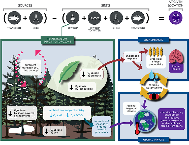
Dry deposition, or removal at the Earth's surface, is a primary sink of ozone in the troposphere where ozone is an air pollutant, greenhouse gas, and central to the atmospheric oxidative capacity. Ozone dry deposition occurring through plant stomata (the pores on leaves controlling gas exchange) damages plants. While the potential for ozone dry deposition to influence air quality, ecosystems, and crop yields has been recognized for decades, mechanistic understanding of ozone dry deposition is incomplete. Figure 1 illustrates processes contributing to ozone dry deposition and how changes in ozone dry deposition impact tropospheric chemistry, air quality, ecosystems, and climate. In this review, we synthesize knowledge of controlling processes, review measurement and modeling approaches, and recommend approaches to close knowledge gaps.
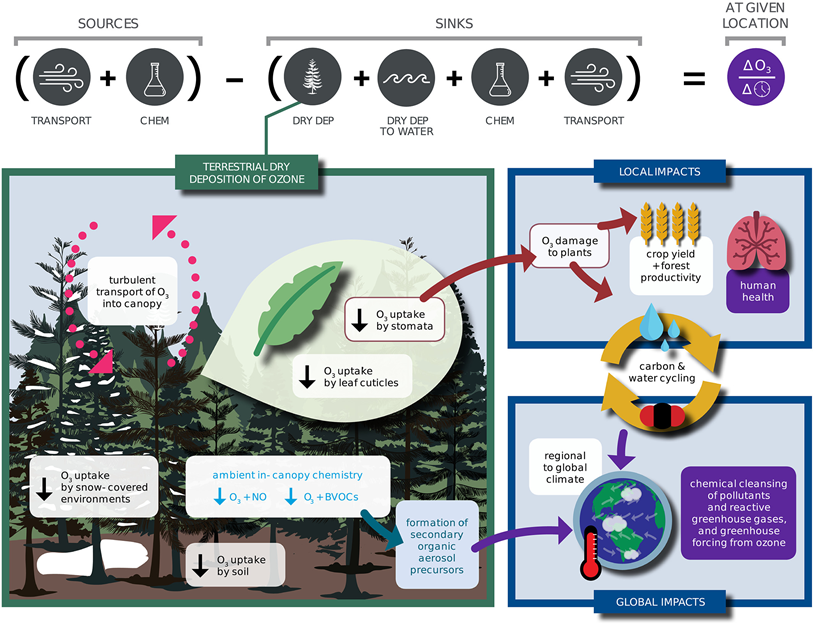
To undergo dry deposition, atmospheric turbulence transports ozone close to a given surface and then ozone must move through the quasi-laminar boundary layer around that surface. The rate of ozone uptake by a particular surface depends on the surface's properties. Ozone dry deposition occurs not only through stomatal uptake but also through other nonstomatal deposition pathways including uptake by leaf cuticles, soil, snow, water, and man-made surfaces. Both surfaces with high-destruction rates (like, vegetation) and spatially extensive surfaces with low destruction rates (e.g., snow and water) are relevant to the tropospheric ozone budget and large-scale ozone pollution.
Quantifying stomatal ozone uptake is not only important for estimating ozone removal but also for understanding the plant response to ozone. Stomatal ozone uptake injures plants by generating reactive oxygen species that can induce cell death and lesions and thus accelerate senescence. Reactive oxygen species also impair photosynthetic enzyme activities, enhance respiration, and interfere with carbon allocation. Ozone injury to plants alters terrestrial carbon and water cycling, which influences boundary-layer meteorology and climate and increases surface ozone due to a reduced stomatal ozone sink.
Numerical simulations of tropospheric ozone, including high ozone pollution episodes and background ozone levels, are sensitive to model descriptions of ozone dry deposition. However, many widely used ozone dry deposition schemes do not represent processes mechanistically or capture observed spatiotemporal variations. Among models, differences are twofold to threefold in estimates of ozone dry deposition for a given location and in estimates of the global annual tropospheric ozone loss through dry deposition. Understanding of the contribution of individual deposition pathways to ozone dry deposition is incomplete but key for building mechanistic representation in the large-scale models used to quantify the effects of ozone dry deposition across Earth systems from hourly to centennial time scales.
Below, we address the following questions:
- What approaches are currently used to measure and model ozone dry deposition?
- What is current understanding of the processes controlling ozone dry deposition based on theory, observations, and modeling?
- What major knowledge gaps and uncertainties exist with respect to (1) and (2)?
- How can we most rapidly advance knowledge of ozone dry deposition and its impacts on air quality, vegetation, and climate?
We examine stomatal, leaf cuticular, soil, and snow deposition pathways, as well as turbulent transport and fast ozone loss through ambient chemistry. Not only is fast chemistry important for building understanding of ozone dry deposition from ozone flux measurements, but it also leads to formation of secondary aerosol precursors. To limit the scope of our review, we do not cover transport through the quasi-laminar boundary layer adjacent to surfaces. However, the magnitude of quasi-laminar transport can widely vary among model parameterizations, and thus, uncertainty in this process may be nonnegligible. Differences across models, the impacts of canopy structure, turbulence, and leaf properties (e.g., aerodynamics, morphology, and presence of water) on transport, and scaling from leaf to canopy should be emphasized in future research. While in this review we discuss the deposition pathways considered to be most important for terrestrial ozone dry deposition impacts on tropospheric chemistry, air quality, and vegetation, we emphasize that better understanding of ozone dry deposition to other terrestrial surfaces, such as urban surfaces, lakes, rivers, branches, and leaf litter, is needed.
2 Measuring Ozone Dry Deposition
2.1 History of Measurements and Survey of Current Data Sets
Methods for field measurement of ozone dry deposition have been available since the 1950s. In the 1950s and 1960s, ozone dry deposition was typically measured using gradient methods during short campaigns. By the 1970s, the eddy covariance (EC) approach—the preferred approach for measuring turbulent fluxes —became possible with fast ozone analyzers deployed on masts and towers and aircraft. Growing recognition of the importance of biogeochemical cycles led to workshops in the late 1970s and 1980s recommending research priorities for fluxes of ozone, carbon dioxide, and other constituents. In particular, a 1987 workshop on trace gas and particle fluxes recommended that future studies “span both diurnal and seasonal cycles” and investigate “surfaces of importance to global budgets”.
Likely as the result of momentum in the research community and support from funding agencies, the number of sites with ecosystem-scale ozone fluxes increased from the late 1980s into the next decade (Figure 2). The first annual record of continuous hourly ozone and carbon dioxide EC fluxes began in the early 1990s at Harvard Forest in the northeastern United States. However, emphasis on ozone dry deposition in the community waned around the millennium, as evident from stabilizing number of sites with measurements after the mid-1990s (very low numbers after 2014 may reflect the time needed to report and analyze data).
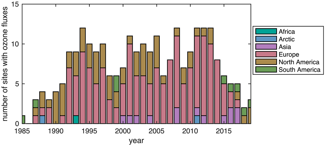
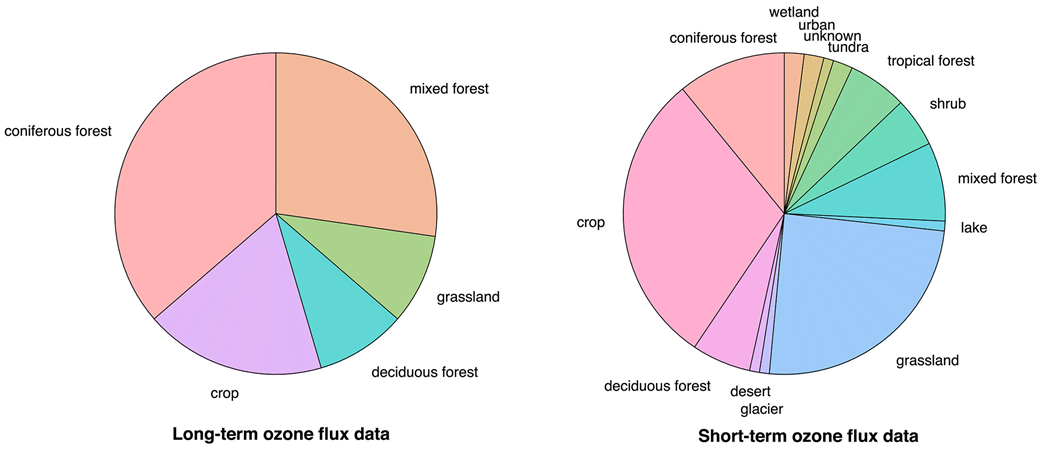
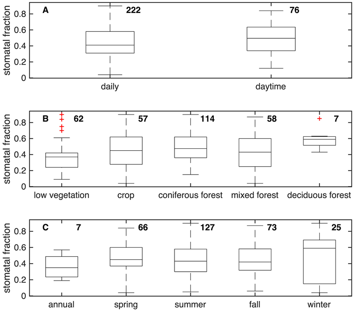
Sites with ozone fluxes primarily reside in Europe and North America (Figure 2), indicating a paucity of knowledge on ozone dry deposition for most parts of the world. More consistent emphasis on ozone fluxes in Europe (Figure 2) may reflect regional initiatives to quantify the impact of ozone on ecosystems. While the observational record captures a variety of land use/land cover (LULC) types, most data are for crops and forests (Figure 3), and the data sets for particularly undersampled LULC types tend to be very short term (i.e., days) (Table A1 in Appendix A).
Advancing understanding of ozone dry deposition requires synthesizing knowledge and testing hypotheses across ozone flux data sets. However, current knowledge does not reflect a meta-analysis of all, or even the majority, of data sets in Table A1. While Table A1 provides a record for future studies to identify potentially available ozone flux data, the lack of a central archive limits efforts to analyze multiple records. Differences in instrumentation, a lack of coordinated protocols across data sets, and in some cases missing complementary measurements also limit the utility of older data and meaningful syntheses across records.
Despite the common emphasis in the 1970s and 1980s on the need to establish long-term flux observations for gases like ozone and carbon dioxide, ozone flux data lag far behind carbon dioxide flux data in the number, data set length, and diversity of sites. Carbon dioxide fluxes are available for around 900 sites for over 7,000 combined site years of data, including many sites with more than a decade of data. In contrast, only 114 sites have ozone fluxes, only 11 sites have more than 5 years of data, and none exceed 15 years (Table A1). There are likely different needs in terms of carbon dioxide versus ozone flux data, but gaining a robust understanding of interannual variability and trends in ozone dry deposition and accurately interpreting the observational anomalies challenging current understanding require long-term data. The recent National Academies of Sciences, Engineering, and Medicine (NASEM, 2016) report on The Future of Atmospheric Chemistry Research also emphasizes the need for long-term fluxes of reactive gases and aerosols.
One issue impeding ozone EC measurements is the fast ozone analyzers meeting the stringent criteria of the EC technique are generally resource intensive to operate. The lack of simple reliable analyzers may in part explain why ozone EC measurements have been limited to research groups with atmospheric chemistry and physics expertise while the ecological community widely adopted carbon dioxide EC, catalyzing the development of a larger network. Motivating the development of new measurement techniques and an observational network is also challenging for an interdisciplinary subject such as ozone dry deposition.
A misconception that the mechanisms controlling ozone dry deposition are well understood may have also contributed to ozone flux measurements losing luster. While the literature widely states that stomatal uptake governs ozone dry deposition over physiologically active vegetation, observationally based estimates of the stomatal fraction of ozone dry deposition show a codominant role for deposition through nonstomatal pathways (Figure 4) with stomatal uptake as 45% of the total on average.
Not only is nonstomatal uptake nonnegligible, but it is also highly variable. Observationally based studies illustrate unexpected variations in nonstomatal deposition in diel cycles including over soil and snow, year-to-year variability, after rain and dew, and spatially. Measurements also show that ambient chemistry with unmeasured biogenic volatile organic compounds (BVOCs) influences ozone flux observations.
Unconstrained variations in ozone dry deposition challenge the ability to attribute changes in tropospheric ozone to other processes (e.g., sources) accurately. Capturing unexpected variability with ozone flux records allows the community to build hypotheses about controlling processes, target laboratory and field measurements and build mechanistic models.
Mechanistic modeling is fundamental for interpreting observed ozone fluxes because the ozone flux integrates many different processes, and techniques to isolate individual processes are limited. For example, isolating nonstomatal deposition and fast in-canopy chemistry from the ozone flux strongly relies on residual analysis, leading to uncertainty in variations and the relative importance of a given process. Together with the statistical power provided by long-term data, mechanistic modeling also informs ozone dry deposition schemes, which currently rely on poorly constrained empirical relationships.
2.2 Measurement Techniques
Here we review approaches for measuring ozone dry deposition. We discuss EC, flux gradient, modified Bowen Ratio, chamber, and isotopic methods. We detail the fast ozone analyzers needed for EC because their cost, maintenance requirements, and limited availability may thwart efforts to measure dry deposition through ozone EC, the most fundamental and direct method for measuring turbulent exchange (e.g., Hicks et al., 1989; Meyers & Baldocchi, 2005).
2.2.1 Micrometeorological Approaches

is ozone concentration; u, v, and w are wind velocity in longitudinal (x), lateral (y), and vertical (z) directions;
is chemical production of ozone;
is chemical loss of ozone; and
is dry deposition of ozone. Overbars represent temporal averages, and primes represent fluctuations from the temporal average.
For this assumption to be valid, equation 3 demonstrates two additional conditions need to be satisfied (or the contributions from each term quantified adequately).
The first condition is negligible ambient ozone chemistry below h
. This is not always true; we further discuss this in section 4.5.
The second condition is stationary ozone concentration on the time frame of the averaging operator
. Storage, or ozone temporarily accumulating within the canopy (i.e., between the ground surface and h), violates this condition. Estimating storage requires ozone concentration measurements at different heights in the canopy (the number of heights needed depends on how much ozone changes vertically). An assumption inherent to using one concentration profile is that the location represents the ecosystem sampled by the vertical turbulent flux measurement. This assumption has been shown to be limited for carbon dioxide.
Storage is considered to be nonnegligible in forest canopies. Not many studies give estimates of ozone storage, but storage tends to overestimate ozone dry deposition in forests during morning and underestimate during evening, with the influence averaging out over a day. Specifically, the bias is <20% at Harvard Forest and Bosco Fontana in Italy but may be ~50% at a tropical forest in Reserva Biológica Jarú.
2.2.1.1 Eddy Covariance
Ozone EC systems are usually custom built by research groups and require atmospheric chemistry and physics expertise. Because there is no formal recipe for their design, we present necessary considerations for ozone and refer the reader to previous reviews on EC.
A first consideration is to measure the vertical wind velocity and ozone concentration at a frequency high enough to resolve the full range of eddies contributing to vertical transport. In particular, the ozone analyzer has to be sufficiently accurate to resolve concentration variability due to turbulence (10–60 Hz) but also ambient chemistry, which may require a faster measurement. Instrument frequency responses can be evaluated by comparing spectra and cospectra for ozone with those for heat and momentum. Derivation of transfer functions based on the cospectra enables correction for any loss of high-frequency contributions.
Current ozone analyzers used for EC are based on chemiluminescence, or light production via chemical reaction, due to their fast response times. While there is a method to correct ozone fluxes measured with an ultraviolet (UV) photometric ozone analyzer, the empirical correction is large, and random uncertainty in the daytime ozone flux is 60% (Wohlfahrt, Hörtnagl, et al., 2009). Reported frequency response corrections from fast ozone analyzers typically range from 5% to 30% (Bauer et al., 2000; Keronen et al., 2003; Horváth et al., 2017; Munger et al., 1996; Plake, Stella, et al., 2015; Zhu et al., 2015).
A second consideration is that duration of the averaging interval must be long enough to sample the slowest turbulent eddies contributing to exchange but short enough that ozone concentration remains stationary. Sampling or random error may be an important contribution to uncertainty in ozone EC. For example, the sampling error ranges from 23% to 33% for one analyzer during different time periods at five sites in the eastern United States (Finkelstein & Sims, 2001) and from 10% to 20% with another analyzer at Hyytiälä in southern Finland (Keronen et al., 2003; Rannik et al., 2009).
Third, there are not currently open-path fast-response ozone analyzers. High instrument flow rates are thus needed to minimize residence time in measurement volumes and ozone loss in the sample stream due to reaction with walls or other compounds, as well as achieve a turbulent flow, which reduces attenuation in the tubing (Lenschow & Raupach, 1991). When the required flow rate is too high for the analyzer to accommodate, excess flow can be pulled through a bypass pump. For pressure-sensitive analyzers (e.g., when the reaction required to detect ozone is sensitive to pressure), linking the bypass flow to a pressure controller may be necessary to maintain constant pressure at the analyzer inlet.
Chemiluminescence analyzers vary by reagent phase: gas, solid (“dry”), and liquid (“wet”). While chemiluminescence analyzers have fast response times and high sensitivity, they can be expensive (gas) or need frequent maintenance and calibration (dry and wet), adding labor costs and down time. Gas chemiluminescence leverages the reactions between ozone and ethene (e.g., Desjardins et al., 1995; Droppo, 1985; Duyzer et al., 1983; Munger et al., 1996) or nitric oxide (NO) (e.g., Bariteau et al., 2010; Eastman & Stedman, 1977; Pearson, 1990; Stedman et al., 1972). While several gas chemiluminescence analyzers were commercially available in the past, to our knowledge, there is only one currently available (Table 1).
| Enviscope GmbH | Schnelle Ozon Sonde | Solid | 10 | Zahn et al. (2012) and Zhu et al. (2015) |
| Sextant | FOS | Solid | 10 | Stella et al. (2012) and Q. Li, Gabay et al. (2018) |
| Ecometrics | Chemiluminescence Ozone Fast Analyser | Solid | 10 | (GFAS clone) https://www.ecometrics.it/cosa-facciamo/338-2/, date of access 10 July 2019 |
| Ecophysics | CLD88 | Gas (NO) | 10 | https://www.ecophysics-us.com/atmospheric-research-products, date of access 10 July 2019 |
Dry chemiluminescence uses a solid dye that emits light upon reaction with ozone. Not requiring toxic (e.g., NO) or flammable (e.g., ethene) compressed gases, dry chemiluminescence is advantageous over gas chemiluminescence. Dry analyzers also can be smaller and only require low power due to the physical configuration of their electronic components and the pumps or fans used to sample air. A coumarin solid dye, which emits a blue light upon reaction with ozone, is typically used for dry chemiluminescence (e.g., Muller et al., 2010). The photomultiplier tubes for detection of blue light are less expensive than the ones for red light needed for other common gas or dry chemiluminescence techniques. A dry analyzer used to be offered by Gesellschaft Für Angewandte Systemtechnik (GFAS) (Güsten et al., 1992; Güsten & Heinrich, 1996). Several groups made or used GFAS clones (e.g., Bauer et al., 2000; Coyle, 2005; Coyle et al., 2009; Cros et al., 2000; Finco et al., 2018; Kurpius et al., 2002; Mészáros, Horváth, et al., 2009). Currently, there are three dry analyzers commercially available, including one GFAS clone (Table 1).
Disadvantages of dry chemiluminescence include degradation of dye-impregnated discs (i.e., loss of ozone sensitivity) such that they need regular replacement (e.g., every few days). There is a 12% daily mean difference between ozone fluxes from a GFAS and a GFAS clone at Easter Bush in southern Scotland (Muller et al., 2010), suggesting analyzer performance and disc stability may be sources of uncertainty in ozone flux data. A new disc preparation method extending disc field stability is described in Ermel et al. (2013) who show high ozone sensitivity can be maintained over threefold more disc ozone uptake. An extended disc stability means measurements can proceed either for longer without maintenance or in higher ozone environments with similar maintenance.
A second ozone analyzer, which can be a commonly used UV absorbance instrument, is always necessary in dry chemiluminescence setups to account for the changing disc sensitivity. Different techniques to calculate an absolute signal can lead to substantially different ozone fluxes, as shown by measurements at Easter Bush (Muller et al., 2010) and a Chinese wheat field (Zhu et al., 2015).
Wet chemiluminescence employs organic liquid dye that emits light upon reaction with ozone (e.g., Drummond et al., 1991; Keronen et al., 2003; Ray et al., 1986; Zona et al., 2014). In principle, wet chemiluminescence is a relative measurement (because the dye degrades), but with a substantial amount of liquid reagent in the bottle used for measurement, it can be considered absolute. The dye does need to recirculate (usually via a peristaltic pump), however, and recirculation often fails when the bottle is not close to full (Keronen et al., 2003). Depending on ozone concentration at the site, the bottle may only need to be refilled every few months to keep it near full though (Keronen et al., 2003).
The need for long-term ambient ozone concentration measurements not requiring much maintenance has driven the market toward instruments inherently too slow for EC. More robust and economical fast analyzers not requiring frequent maintenance or involving toxic or flammable consumables or compressed gases will enable more ozone EC measurements and thus faster progress toward improved understanding of ozone dry deposition.
2.2.1.2 Flux Gradient
The eddy diffusivity for sensible heat can be calculated by employing Monin-Obukhov Similarity Theory (MOST) (Businger et al., 1971; Högström, 1988). However, MOST does not hold in the roughness sublayer above vegetation (Raupach, 1979), which can extend higher than double the vegetation height (e.g., Cellier & Brunet, 1992; Harman & Finnigan, 2007; Thom, 1975). Most observed gradients are located below this height. Additionally, ozone is reactive, and ambient chemistry may perturb the ozone gradient so assuming the eddy diffusivity for ozone is equal to that for heat is not always valid (Fitzjarrald & Lenschow, 1983; Lenschow, 1982; Vilá-Guerau de Arellano & Duynkerke, 1992).
Using a single analyzer with switching or moveable inlets to sequentially sample concentrations at different heights for the ozone gradient measurement is preferred over separate analyzers for the different heights because the latter requires effort to eliminate biases between the analyzers. However, when the measurements are not simultaneous (i.e., one analyzer is used at multiple heights), then the gradient needs to be stable over the time required to obtain measurements at both heights. Otherwise, there needs to be a correction for sequential sampling.
Inferring accurate ozone fluxes using the flux gradient technique is also challenging because ozone differences between the two heights may be very small and challenge the resolution and accuracy of the instrument (Businger, 1986). Maximizing the vertical distance between top and bottom heights to get larger differences helps (Arya, 2001), but both measurements must be in the surface layer with comparable footprints. Comparison of ozone EC and gradient fluxes over several ecosystems suggests fluxes and vd from the flux gradient technique may be biased and not represent variations accurately (Duyzer & Westrate, 1995; Loubet et al., 2013; Mikkelsen et al., 2000; Muller et al., 2009; Z. Y. Wu et al., 2015).
2.2.1.3 Modified Bowen Ratio
The concentrations of ozone and the reference quantity
are from measurements at the same heights in the surface layer. The modified Bowen Ratio technique may be advantageous over the flux gradient technique because the modified Bowen Ratio technique does not directly require turbulent diffusivity estimates. While commonly used ozone UV absorbance instruments are likely adequate for this technique, this method requires detection of likely small gradients in ozone and the reference quantity. Previous work suggests substantial biases (50–100%) in ozone fluxes estimated with the modified Bowen Ratio technique with carbon dioxide fluxes relative to ozone EC at Harvard Forest (Z. Y. Wu et al., 2015).
2.2.2 Chamber Methods
Chamber methods are employed to isolate ozone uptake to foliage, soil, water, and other surfaces in the field (Almand-Hunter et al., 2015; Altimir et al., 2002; Fumagalli et al., 2016; Gut et al., 2002; Horváth et al., 2006; Kaplan et al., 1988; Kirkman et al., 2002; Meixner et al., 1997; Pilegaard, 2001; Remde et al., 1993; Tong et al., 2011; Unsworth et al., 1984; Wieser et al., 2012). However, previous work largely focuses on soil NO emissions (e.g., Gut et al., 2002; Horváth et al., 2006; Kaplan et al., 1988; Kirkman et al., 2002; Meixner et al., 1997; Remde et al., 1993) or plant responses to ozone (e.g., Tong et al., 2011; Wieser et al., 2012) rather than ozone deposition processes.
For an open chamber, air is generally drawn into the chamber, and the ozone concentration difference between the inlet and outlet is measured with a slow ozone instrument. The uptake rate to the surface is determined from the concentration difference, the known flow rate into the chamber, and volume of the chamber.
We emphasize the value of chamber methods for gaining mechanistic understanding of ozone dry deposition (e.g., Altimir et al., 2006; Fumagalli et al., 2016). However, we note that chamber footprint is small (i.e., on the order of a meter or less), chambers modify microclimate, and ozone chemistry may occur in the chamber air or with chamber walls and tubing (Breuninger et al., 2012; Pape et al., 2009). In the field, multiple chambers are necessary to account for inhomogeneity across a wider area (e.g., the footprint of a flux tower) as well as understand the robustness of observed dependencies on environmental conditions.
The strength in using chamber measurements to separate the canopy portion of the ozone flux from the ground ozone uptake (see equation 4) (e.g., Duyzer et al., 2004; Finco et al., 2018; Rummel et al., 2007) or to serve as a surrogate to ozone EC (Almand-Hunter et al., 2015; Plake, Stella, et al., 2015) hinges on the ability to obtain an estimate spatially representative of the ecosystem, to remove the effects of turbulent transport modified by the chamber, and to estimate in-canopy turbulent transport and the contribution from fast ambient chemistry to the ecosystem-scale ozone fluxes.
2.2.3 Isotopic Methods
Isotopic experiments in the laboratory and field may be able to pinpoint the primary sites of ozone surface reactions and thus improve understanding of ozone deposition pathways (Subke et al., 2009; Toet et al., 2009). Subke et al. (2009) present a method for adding 18O into an electric discharge ozone generator and using a silica gel to separate 18O ozone from 18O O2. However, 18O from the generated ozone leads to 18O enriched water vapor as well as other gases (e.g., O2) that do not necessarily remain on a surface, complicating estimates of deposited ozone (Toet et al., 2009). The authors conclude that better understanding of the reactions determining loss of 18O ozone into other gases is needed for this technique to be useful for constraining ozone deposition pathways.
3 Modeling Ozone Dry Deposition Using Resistance Networks
We present common resistance network approaches for parameterizing ozone dry deposition in models considering vegetation as one big leaf and in models considering vertical variation in plant canopy structure. In general, resistance network approaches have many strengths. For example, resistance approaches are appropriate for modeling at different scales, simple, and adaptable, and allow for representing individual processes.
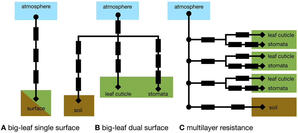
The big-leaf resistance network structure varies across different dry deposition schemes. For example, Wesely (1989) consider a bulk quasi-laminar boundary layer resistance for soil and leaves, which is added in series with the bulk ra, whereas Massman (2004) consider different quasi-laminar boundary layer resistances for soil versus leaves.
To calculate vd with this approach, the above rsurf parameterization needs to be embedded into a model considering ozone turbulent transport among canopy layers and between hc and h. Turbulent transport could be simulated with a resistance approach or more explicitly.
Most ozone dry deposition schemes deployed in regional and global models use big-leaf approaches. Multilayer resistance approaches exist (e.g., Duyzer et al., 2004; Fares et al., 2019; Ganzeveld et al., 2002; Launiainen et al., 2013; Meyers et al., 1998; Potier et al., 2015; Wolfe & Thornton, 2011; P. T. Zhou et al., 2017) but mostly are used in single-point models for interpreting field observations rather than modeling regional-to-global ozone dry deposition. An advantage of the multilayer approach is that the ozone continuity equation can be calculated at every height and thus the influence of in-canopy chemistry (e.g., Ashworth et al., 2015; Wolfe et al., 2011) or turbulence (e.g., Chang et al., 2018; Patton et al., 2016; Pyles et al., 2000) explicitly resolved. We refer to the approach where the ozone mass continuity equation is solved at each height as a multilayer canopy model. To our knowledge, in-canopy chemistry has never been explicitly considered in a big-leaf framework although empiricism in model development may have led to implicit inclusion (Wolfe et al., 2011).
4 Theory, Models, and Observations of Terrestrial Ozone Deposition Pathways and Related Processes
We review ozone dry deposition to plant stomata (section 4.1), leaf cuticles (section 4.2), soil (section 4.3), and snow-covered surfaces (section 4.6). We also review turbulent transport (section 4.4) and ambient chemistry (section 4.5), presenting these sections before the section on deposition to snow-covered surfaces due to our focus on turbulence and chemistry in plant canopies. In all sections, we discuss modeling and measurement techniques. For sections on deposition to cuticles, soil, and snow-covered surfaces, we synthesize understanding of these processes based on laboratory and field observations and theory. For sections on stomatal deposition, turbulence, and fast ambient chemistry, we highlight advances in understanding pioneered by the fields of plant physiology/ecology, boundary-layer meteorology, and atmospheric chemistry, respectively, and identify steps needed to advance knowledge of the process as related to ozone dry deposition.
4.1 Stomata
rb,leaf is the resistance to transport through the quasi-laminar boundary layer between the leaf and outside air; rstom is the resistance to gaseous diffusion through stomatal pores; and rmeso is the resistance to ozone reaction inside the leaf. The inverse of rstom is stomatal conductance (gs). While a mesophyll resistance (i.e., rmeso) is the conventional way of describing that reactions destroying ozone within the leaf may limit Fstom, ozone is not primarily destroyed inside the leaf by reactions with the mesophyll tissue. Despite rmeso being a misnomer, we retain the terminology for consistency with previous work (e.g., Wesely, 1989).
Observational approaches and prognostic models for rstom are typically for water vapor. To obtain an estimate of the resistance to ozone diffusion through stomatal pores, rstom for water vapor is multiplied by the ratio of the diffusivity of water vapor in air to the diffusivity of ozone in air. The current estimate of this ratio is 1.61 (Massman, 1998). The assumption inherent to this approach is proportionality between ozone diffusing inward through stomata and water vapor diffusing outward. One limitation of this assumption is that collisions between ozone and water vapor molecules may lead to an error of 4–10% in estimates of the stomatal ozone flux (Uddling et al., 2012).
A widely used assumption is that reactions inside the leaf do not limit stomatal ozone uptake (i.e., negligible rmeso). While some laboratory studies (Laisk et al., 1989; Omasa et al., 2000; S. Sun, Moravek, von der Heyden, et al., 2016; Wang et al., 1995) and the modeling study of Plöchl et al. (2000) suggest this assumption holds, the findings of other laboratory studies and the modeling study of Tuzet et al. (2011) suggest otherwise. In particular, laboratory findings of nonlinear relationships between stomatal uptake of water vapor and stomatal uptake of ozone (Eller & Sparks, 2006; Fares et al., 2007; Fares, Park, et al., 2010; Loreto & Fares, 2007; Tuzet et al., 2011) may imply nonnegligible resistance to ozone reaction inside the leaf. Nonetheless, separating ozone destruction inside the leaf from gs, cuticular ozone uptake, and gas-phase ozone loss is challenging. We recommend future studies further investigate ozone destruction inside the leaf and its influence on stomatal ozone uptake.
In the rest of this section, we highlight common observational constraints on gs (section 4.1.1) and prognostic gs models (section 4.1.2). We discuss leaf, tree, and ecosystem-scale observational approaches. Note we say observational constraints or approaches because gs is not typically measured directly. For prognostic gs modeling, common mechanistic and empirical approaches are highlighted. We also review how the stomatal ozone sink may influence itself through ozone plant damage (section 4.1.3).
4.1.1 Measuring Stomatal Conductance at Leaf, Tree, and Ecosystem Scales
Leaf-level observational constraints typically inform mechanistic and empirical prognostic gs models. Leaf-level gs is inferred from a leaf diffusion porometer or gas exchange system, which record changes in humidity or maintain constant water vapor to infer transpiration. To obtain gs, transpiration is divided by the vapor pressure deficit between the substomatal cavity of the leaf and porometer chamber. To calculate vapor pressure deficit, the air inside the leaf is assumed to be saturated. A recent study using carbon and water isotopes challenges this assumption, finding subsaturation in two conifer species under moderate to high atmospheric vapor pressure deficit and a resulting bias in the inferred gs (Cernusak et al., 2018). Whether subsaturation inside the leaf occurs more broadly is unknown.
Ecosystem-scale observational gs constraints are often used for directly interpreting ozone turbulent flux measurements and estimate the ecosystem-scale stomatal ozone uptake. We discuss multiple methods of inferring ecosystem-scale gs because we recommend using multiple independent approaches to quantify ecosystem-scale gs due to uncertainties across approaches. Ideally, agreement among approaches would be used to draw robust conclusions.
The first ecosystem-scale method employs water vapor EC fluxes and is the most popular method for estimating the ecosystem-scale stomatal ozone uptake. In this method, water vapor fluxes are inverted assuming Fick's law to obtain a surface conductance for water vapor. The intricacies of this method, described below, result in several ways of applying it (e.g., Gerosa et al., 2007).
The surface conductance for water vapor is not exactly gs because surface conductance includes contributions from in-canopy turbulent transport of water vapor (Baldocchi et al., 1987; Baldocchi et al., 1991; Paw U & Meyers, 1989; Raupach & Finnigan, 1987) and evaporation from soil and vegetation (Baldocchi et al., 1987; Baldocchi & Meyers, 1998; Raupach & Finnigan, 1987) in addition to gs. The contribution of evaporation is undesirable in estimating stomatal ozone uptake because evaporation is not directly related to ozone dry deposition. While advances with respect to the ecosystem-scale transpiration fraction of evapotranspiration (e.g., Stoy et al., 2019) will help estimates of surface conductance more strictly represent gs, there is still the issue that surface conductance includes the contribution of turbulent transport of water vapor through the canopy. Assuming similar in-canopy concentration profiles of ozone and water vapor, the contribution of in-canopy turbulence to the surface conductance may be desirable in an ecosystem-scale estimate of gs. However, the safety of the assumption of similar ozone and water vapor in-canopy profiles and thus transport needs to be evaluated.
Inverting the water vapor EC flux via Fick's law for surface conductance requires an ecosystem-scale estimate of water vapor inside the leaf. The assumption for estimating this is that leaf air is saturated, which may be problematic as suggested by leaf level measurements (e.g., Cernusak et al., 2018), and requires an estimate of ecosystem-scale leaf temperature (more commonly, canopy skin temperature). Because canopy skin temperature constraints are not usually available, most inversion approaches include an approximation depending on sensible heat flux, which can be (and previously had to be) inferred from the surface energy budget (i.e., by subtracting the ground heat flux and latent heat flux from net radiation). Not only does the lack of surface energy balance closure in EC measurements (Foken et al., 2010; Wilson & Baldocchi, 2000) suggest errors in inferring sensible heat flux from energy balance, but including latent heat flux in an equation for latent heat flux introduces circularity (Wohlfahrt, Haslwanter, et al., 2009). Modern sensible heat flux measurements avoid the need to estimate sensible heat flux, and thus, methods that incorporate the measured sensible heat flux should be used over methods that estimate the sensible heat flux. New canopy skin temperature measurements (e.g., Kim et al., 2016) may lead to even more accurate estimates of surface conductance.
Ecosystem-scale fluxes of other gases should be used to complement ecosystem-scale gs estimates from water vapor fluxes (e.g., Clifton et al., 2019). Carbon dioxide fluxes can be used to constrain gs through empirical or semiempirical modeling (see section 4.1.2) but require uncertain estimates of respiration (e.g., Wehr et al., 2016) to infer net photosynthesis. Carbonyl sulfide fluxes (e.g., Whelan et al., 2018) are used to validate an empirical gs model for Harvard Forest (Wehr et al., 2017; Wehr & Saleska, 2015) based on findings that they represent ecosystem-scale gs (Commane et al., 2015). Whether this approach transfers readily from Harvard Forest to other locations remains to be established.
Sap flow measurements on individual trees can also be useful for estimating the stomatal ozone flux (Fares et al., 2012; Goldstein, 2003; Matyssek et al., 2004; Nunn et al., 2010; Wieser et al., 2003, 2006) because sap flow isolates transpiration's contribution to the total water vapor flux. However, constraining ecosystem-scale gs with sap flow requires nontrivial scaling from individual trees to the ecosystem. At a mixed forest in Europe, the stomatal fraction of the ozone flux from sap measurements is 42% lower than inverting ecosystem-scale water vapor fluxes (Nunn et al., 2010). While differences may be due to evaporation from foliage and soil influencing the inversion of ecosystem-scale water vapor flux, uncertainties in sap flow measurements and scaling techniques (e.g., Poyatos et al., 2016) may also contribute to differences between approaches.
4.1.2 Modeling Stomatal Conductance
The most popular prognostic gs models in dry deposition schemes are empirical and closely adhere to the Jarvis (1976) multiplicative approach (e.g., Emberson, et al., 2000; Wesely, 1989). In the Jarvis approach, a prescribed maximum gs is multiplied by several factors, and each factor is a function of a particular environmental condition. The conditions may be meteorological or biophysical (e.g., soil moisture and leaf age). The Jarvis type of model is informed by leaf level and sometimes ecosystem-scale observational gs constraints (e.g., Büker et al., 2007, 2012; Kelliher et al., 1995).
An increasingly common method for prognostic gs modeling is coupling gs with net photosynthesis (Anet) (hereafter, Anet-gs model), providing an estimate of carbon dioxide exchange across stomata driven by the carbon supply and demand for photosynthesis. In an Anet-gs model, gs is modeled according to a relationship with Anet (Miner et al., 2017; S. C. Wong et al., 1979) that varies with some metric of humidity, as constrained by leaf-level data (Ball et al., 1987; Leuning, 1995; Medlyn et al., 2011). Recent work assigns a physical basis to this relationship by reconciling mechanistic and empirical approaches with optimization theory for maximizing carbon gain and minimizing water loss (Cowan & Farquhar, 1977; Y. S. Lin et al., 2015; Medlyn et al., 2011). However, whether stomata function optimally as assumed under this particular theory is uncertain (e.g., Buckley & Mott, 2013; C. Lin et al., 2018; Sperry et al., 2017; Wolf et al., 2016; S. Zhou et al., 2013).
In general, whether modeled through empirical or mechanistic prognostic approaches, gs is calculated for a single leaf and scaled to the ecosystem by multiplying leaf-level gs by leaf area index (LAI) or using canopy scaling factors or a multilayer canopy or resistance model. It is uncertain which scaling approach best estimates gs.
While some dry deposition schemes employ Anet-gs models (Charusombat et al., 2010; Clifton, 2018; Hollaway et al., 2016; M. Lin et al., 2019; Ran et al., 2017; Val Martin et al., 2014), the Jarvis type of model remains ubiquitous (e.g., Emberson, et al., 2000; Hardacre et al., 2015). Anet-gs models are more closely based on physiological principles, but the simplicity, adaptability, and computation efficiency of the Jarvis approach make it attractive for many applications. However, the Jarvis approach requires tuning for the ecosystems and environmental conditions represented, and its success is limited by dearth of data for many ecosystems (e.g., tropical forests) and conditions. Nonetheless, Anet-gs models are semiempirical in that they require one to a few parameters to be defined (Franks et al., 2018; Y. S. Lin et al., 2015; Medlyn et al., 2011; Miner et al., 2017). Both model types are typically tuned with leaf-level data due the historical lack of ecosystem-scale data. Recent efforts to tune models with ecosystem-scale measurements (e.g., J. Li, Duan, et al., 2018; Raoult et al., 2016), such as latent heat and carbon dioxide fluxes, can complement leaf-level approaches by allowing for insight into what happens at larger scales.
To evaluate the strengths and weaknesses of prognostic gs models in simulating stomatal ozone uptake, the community would benefit from better understanding of model sensitivities to parameters and variables as well as their physiological realism. For example, connections between gs and soil moisture and the ability of models to capture such connections (e.g., Anderegg et al., 2017; Bonan et al., 2014; Kennedy et al., 2019; Verhoef & Egea, 2014; S. Zhou et al., 2013) may be critical for capturing stomatal ozone uptake.
4.1.3 Ozone Damage to Plants, as Relevant for Stomatal Uptake of Ozone
Ozone damage to plants may lead to myriad ecosystem responses. Here we focus on the direct influence of ozone on gs and thus stomatal ozone dry deposition.
Stomatal ozone uptake changes gs through both short-term and long-term responses. In the short term, stomatal ozone uptake decreases gs by changing guard cell turgor pressure and signaling pathways (Freer-Smith & Dobson, 1989; Hassan et al., 1994; Maier-Maercker & Koch, 1991; Manes et al., 2001; Mills et al., 2009; Torsethaugen et al., 1999).
In the long term, the mean gs response to stomatal ozone uptake across plant physiological studies is a decrease (Lombardozzi et al., 2013). However, both gs increases and decreases are observed. For example, stomatal ozone uptake can lead to reduced photosynthetic efficiency, which increases internal carbon dioxide and signals stomatal closure (Calatayud et al., 2007; Farage et al., 1991; Herbinger et al., 2007; Manes et al., 2001; Noormets et al., 2001; Paoletti & Grulke, 2005; Reich, 1987). On the other hand, stomatal ozone uptake can lead to gs increases in the long term through decreased sensitivity to abscisic acid (Mills et al., 2009), which alters stomatal cell ion exchange (Manes et al., 2001; Torsethaugen et al., 1999), and the collapse of epidermal cells surrounding guard cells (Hassan et al., 1994), which can lead to sluggish stomatal responses to external stimuli (Freer-Smith & Dobson, 1989; Maier-Maercker & Koch, 1991; Manes et al., 1998, 2001; McLaughlin et al., 2007; Paoletti, 2005; Paoletti & Grulke, 2010). Stomatal ozone uptake may also cause early and a more rapid onset of senescence (e.g., Ainsworth et al., 2012), which reduces gs through growing season length and physiologically active LAI.
Two types of model parameterization allow for stomatal ozone uptake to influence itself. In the first type, a response integrated across several physiological processes is used to parameterize impact of ozone on a single physiological process (Clark et al., 2011; Sitch et al., 2007; Yue & Unger, 2014). For example, the observed effect of stomatal ozone uptake on plant biomass or crop yield may be equated to the ozone impact on photosynthesis in models and parameterized accordingly, and thus, any impact on stomatal ozone uptake is due to ozone's parameterized impact on photosynthesis (e.g., Sitch et al., 2007).
The second type of model considers the ozone impact on the same physiological process considered in the observational evidence (Ewert & Porter, 2000; Deckmyn et al., 2007; Lombardozzi, Levis, et al., 2012; Lombardozzi, Sparks, et al., 2012; Lombardozzi et al., 2015; Martin et al., 2001; Tao et al., 2017). For example, Lombardozzi et al. (2013) investigate the effects of cumulative stomatal ozone uptake on gs versus photosynthesis with a meta-analysis of published chamber data. Finding differing observed effects on the two processes, consistent with other work (e.g., Koch et al., 1998; Paoletti & Grulke, 2010), Lombardozzi et al. (2013) parameterize the effect of the cumulative stomatal ozone uptake on each process separately.
Another difference across models parameterizing ozone damage with stomatal ozone uptake is whether damage is tied to the instantaneous or cumulative stomatal ozone uptake. There are a few models, most commonly for crops, considering both instantaneous and cumulative stomatal uptake (Emberson et al., 2018; Ewert & Porter, 2000; Tao et al., 2017). Plant damage is often assumed more closely related to cumulative, rather than instantaneous, stomatal ozone uptake (Ducker et al., 2018; Massman et al., 2000; Matyssek et al., 2004).
Stomatal ozone uptake does not account for plant abilities to cope with the oxidative stress that ozone causes (i.e., detoxify). Detoxification ability controls the plant sensitivity to ozone and thus determines the ozone plant injury (e.g., Matyssek et al., 2008; Musselman et al., 2006). Detoxification is often simulated by assuming a constant threshold of stomatal ozone uptake below which damage does not occur due to detoxification. Detoxification is highly uncertain and may vary with environmental variables and come at a cost to the plant (U.S. EPA, 2006; Ainsworth et al., 2012; Ainsworth, 2017; Musselman et al., 2006; Matyssek et al., 2008).
Current knowledge of the effects of stomatal ozone uptake on gs at large scales (e.g., ecosystem or region) is largely based on scaling up leaf-level effects (Massman et al., 2000; Matyssek et al., 2008). Limited leaf-level data (e.g., most data are for temperate species) and lack of clear response across existing data sets (e.g., Lombardozzi et al., 2013) limit the fidelity of given empirical parameterization. In general, large-scale responses to stomatal ozone uptake are poorly understood and not widely evaluated given the paucity of observational constraints on ozone damage at larger scales. Understanding ecosystem abilities to detoxify is sorely needed to pinpoint stomatal ozone uptake's influence on itself.
4.1.4 Main Takeaways
- Water vapor EC fluxes are typically used to constrain ecosystem-scale gs, but multiple independent observational approaches are needed and ideally agreement among them would be used to draw robust conclusions.
- Anet-gs models represent current mechanistic understanding, but how much Anet-gs models improve gs estimates over widely used empirical approaches is uncertain.
- Identification of the key parameters to which prognostic gs models are most sensitive and an understanding of the physiological realism of modeled sensitivities are needed.
- Ecosystem-scale constraints on stomatal ozone uptake and the ecosystem's ability to detoxify are missing but key for understanding the influence of stomatal ozone uptake on itself.
4.2 Leaf Cuticles
4.2.1 Controls on Ozone Dry Deposition to Leaf Cuticles: Field, Modeling, and Laboratory Evidence
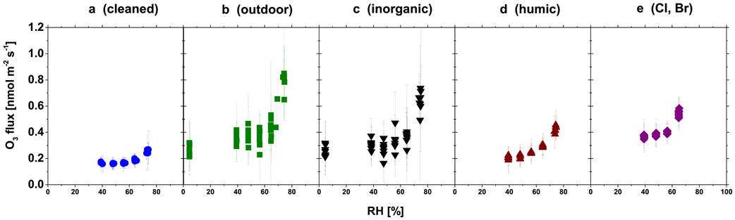
The following synthesis suggests aqueous heterogeneous chemistry is the primary mechanism controlling ozone dry deposition to leaf cuticles. Direct constraints on cuticular ozone uptake are slim but insightful. For example, ozone and carbon dioxide leaf uptake measured with chambers at Hyytiälä provide strong evidence for a dependence of cuticular ozone uptake on relative humidity (Altimir et al., 2006). A laboratory study that induced stomatal closure in young trees by treating leaves with abscisic acid also shows increases in ozone uptake with relative humidity (S. Sun, Moravek, Trebs, et al., 2016) (Figure 6). Increases in cuticular uptake with humidity suggest aqueous ozone-destroying chemistry on the cuticle; liquid surface films form when humidity increases because there is absorption of water to the leaf surface, capillary condensation, or deliquescence of deposited particles (Burkhardt & Eiden, 1994; Burkhardt & Hunsche, 2013; Eiden et al., 1994).
Several field studies report increases in inferred nonstomatal uptake over vegetation with relative humidity, providing evidence that aqueous surface chemistry on leaves may be important at ecosystem scales (Altimir et al., 2006; Clifton et al., 2019; Lamaud et al., 2009; Q. Li, Gabay et al., 2018; Neirynck & Verstraeten, 2018; Rannik et al., 2012; L. Zhang et al., 2002). However, at some field sites, nonstomatal uptake increases with humidity at high humidity but decreases with humidity at low humidity (Coyle et al., 2009; Hogg et al., 2007). This diverging behavior may reflect a change in the mechanism controlling cuticular uptake with thermal decomposition dominating at lower humidity (Coyle et al., 2009; Grøntoft et al., 2004; Pöschl & Shiraiwa, 2015). In general, the degree to which ecosystem-scale nonstomatal uptake estimates represent cuticular uptake is uncertain because other processes, such as ozone uptake by soil and ambient chemistry, cannot always be discounted. Additionally, imperfect estimates of stomatal deposition and transport imply at least some error in residual nonstomatal deposition estimates.
A recent review of ozone dry deposition to building surfaces concludes the influence of relative humidity on ozone uptake is uncertain (Shen & Gao, 2018). It may be that only some ozone-destroying surface reactions are expedited in water films and water films only form easily on some surfaces. Increased cuticular uptake at higher humidity may also be associated with stomatal exudation of reactive compounds when leaves are wet (Potier et al., 2017). For example, water around stomata can act as a bridge into saturated stomatal pores (Burkhardt, 2010), and stomata may leach ascorbate compounds into the water on the cuticle. If ozone destruction on cuticles is limited by ascorbate flowing out of stomata when leaves are wet, then a fundamental question is how much leakage occurs.
In their laboratory study examining ozone uptake to aluminum, stainless steel, beeswax, and hydrocarbon wax, Cape et al. (2009) find an Arrhenius-like dependence of ozone uptake on temperature and suggest a role for thermal decomposition of ozone when ozone deposits to leaf cuticles. There is some field evidence for this hypothesis in dry conditions, as discussed above. However, increases in temperature only lead to small increases in ozone uptake to building surfaces (Shen & Gao, 2018). In general, thermal decomposition of ozone on a given surface depends on the surface area and activation energy, which varies across materials (e.g., Cape et al., 2009). Whether thermal decomposition plays a role in governing cuticular ozone uptake needs to be better understood.
While light-mediated ozone destruction on cuticles received attention in previous reviews on ozone dry deposition (e.g., Fowler et al., 2009; Ganzeveld et al., 2015; Tuovinen et al., 2009), evidence for the importance and occurrence of this pathway is minimal. In brief, Coe et al. (1995) find a diel cycle in nonstomatal deposition inferred from field measurements. The hypothesis that photochemistry on the leaf surface causes this diel cycle is given attention on the basis of Rondón (1993), an unpublished laboratory study. A more recent laboratory study finds similar cuticular ozone uptake for light and dark conditions (S. Sun, Moravek, Trebs, et al., 2016), suggesting cuticular uptake is unlikely to be related to photochemistry.
High vd after rain and dew observed in field studies is often attributed to increases in cuticular uptake (Altimir et al., 2006; Finkelstein et al., 2000; Fuentes et al., 1992; Grantz et al., 1995, 1997; Lamaud et al., 2002; Potier et al., 2015; Turnipseed et al., 2009). Increases in ozone dry deposition on wet leaves in the laboratory (Fuentes & Gillespie, 1992) and in a field chamber experiment after spraying the grass in the chamber with water (Pleijel et al., 1995) are also attributed to increases in cuticular uptake. While there are fairly consistent increases in vd over vegetation after rain and dew across field studies (Table 2), whether observed responses truly indicate changes in cuticular uptake remains an open question. For example, there may be changes in gs after rain (e.g., Clifton et al., 2019) or emissions of highly reactive species that influence the observed ozone flux (e.g., Altimir et al., 2006; Clifton et al., 2019; Turnipseed et al., 2009).
Table 2. Summary of Field Studies Reporting Changes in Ozone Dry Deposition After Rain and Dew
| Bondville (40.05°N, 88.37°W) | 2 months of ozone EC fluxes | Maize | Increase | Increase | L. Zhang et al. (2002) |
| Camp Borden (44°19′N, 79°56′W) | 5 days of ozone EC fluxes | Temperate deciduous forest | Increasea | Increasea | Fuentes et al. (1992) |
| 2 months of ozone EC fluxes | Decrease (day), no change (night) | Increase (episodic), no change (systematic) | Padro (1994) | ||
| CODE cotton (36°48′50″N, 120°40′38″W) | 1 month of ozone EC fluxes | Cotton | No changea | Massman et al. (1994) | |
| Decrease | Grantz et al. (1997) | ||||
| CODE vineyard (36°51′36″N, 120°6′7″W) | 1 month of ozone EC fluxes | Vineyard | No changea | Massman et al. (1994) | |
| Increase | Grantz et al. (1995) | ||||
| Flanders (51°18′N, 4°31′E) | 10 years of ozone fluxes from flux gradient technique | Temperate deciduous forest | Increase | Increase | Neirynck and Verstraeten (2018) |
| Grignon (48.84422°N, 1.95191°E) | 5 months of ozone EC fluxes from 3 years each | Wheat | Increase | Increase | Potier et al. (2015) |
| Harvard Forest (42.53°N, 72.18°W) | 4 months of ozone EC fluxes from 11 years each | Temperate deciduous forest | Increaseb | Clifton et al. (2019) | |
| Hyytiälä (61.85°N, 24.28°E) | 6 months of ozone EC fluxes from 2 years each | Boreal forest | Increase | Altimir et al. (2006) | |
| Kane Experimental Forest (41.595°N, 78.766°W) | 4 months of ozone EC fluxes | Temperate deciduous forest | Increaseb | Clifton et al. (2019) | |
| 7 months of ozone EC fluxes | Decrease (day), increase (night) | Increase (day), no change (night) | Finkelstein et al. (2000) | ||
| Increase | Increase | L. Zhang et al. (2002) | |||
| Les Landes (44°12′N, 0°42′W) | 2 months of ozone EC fluxes from 2 years | Temperate coniferous forest | Increase | Lamaud et al. (2002) | |
| Nashville (36.65°N, 87.03°W) | 5 months of ozone EC fluxes | Soybean | Decrease | L. Zhang et al. (2002) | |
| Niwot Ridge (40.03°N, 105.55°W) | 3 to 7 months of ozone EC fluxes from 4 years each | Subalpine coniferous forest | increase | Turnipseed et al. (2009) | |
| Rush | 1 day of ozone EC fluxes | Senescent maize | Decreasea | Wesely et al. (1978) | |
| Sand Flats State Forest (43.565°N, 75.238°W) | 4 months of ozone EC fluxes | Temperate mixed forest | Increaseb | Clifton et al. (2019) | |
| 6 months of ozone EC fluxes | Increase (day), no change (night; high LAI), increase (night; low LAI) | Increase (day), no change (night; high LAI), increase (night; low LAI) | Finkelstein et al. (2000) | ||
| Increase | Increase | L. Zhang et al. (2002) | |||
| Sand Mountain (34.29°N, 85.97°W) | 2 months of ozone EC fluxes | Pasture | Decrease (day), increase (night) | Increase | L. Zhang et al. (2002) |
| Sangamon, Illinois | 2 days of ozone EC fluxes | Healthy maize | Decreasea | Wesely et al. (1978) |
- a Findings may be particularly uncertain due to low signal-to-noise ratio or authors do not calculate systematic differences (e.g., average over composites).
- b Study does not attribute changes, or all changes, to cuticular uptake.
4.2.2 Composition of the Leaf Cuticle
Composition of the cuticular surface likely determines ozone reactivity. Cuticular composition and thus reactivity may reflect deposited aerosols, the cuticular wax itself, and/or compounds exuded from the plant, but the relative importance of each source of reactivity is uncertain and may vary in space and time. Different wetting mechanisms may alter cuticular composition and thus ozone uptake. For example, rain may wash leaves of compounds (e.g., Xu et al., 2017; L. Zhang et al., 2019) with which ozone can react. Deliquescent salts on cuticles may also increase ozone solubility compared to pure water (e.g., Rischbieter et al., 2000). Below we discuss evidence for each source (deposited aerosols, cuticular wax, and exuded compounds) contributing to ozone reactivity. We find that the dominant reactivity sources on cuticles needs to be established.
Depending on leaf size and shape, up to 50 μg cm−2 of aerosols can accumulate on leaves (Burkhardt, 2010; Popek et al., 2013; Sæbø et al., 2012). In the laboratory study of S. Sun, Moravek, Trebs, et al. (2016), ozone uptake is highest for leaves either exposed to outdoor air or sprayed with a solution containing major inorganic components of typical continental aerosols relative to the other treatments (Figure 6), suggesting cuticular uptake through reaction with deposited aerosols may be important. However, evidence from kinetic studies on soot, mineral dust, and proxies for organic aerosols shows rapid declines in ozone uptake after high initial uptake (Chapleski et al., 2016; Disselkamp et al., 2000; Hanisch & Crowley, 2003; Karagulian & Rossi, 2006; McCabe & Abbatt, 2009), implying persistent ozone uptake requires sustained aerosol deposition to cuticles. The exception is uptake by organic photosensitizers (e.g., humic acid) in light (D'Anna et al., 2009; Jammoul et al., 2008).
Cuticular waxes mostly contain compounds derived from long-chain fatty acids unreactive with ozone but can contain unsaturated compounds (Buschhaus & Jetter, 2012; Jetter et al., 2006; Yeats & Rose, 2013) reactive with ozone. Clean cuticles have low but nonnegligible ozone uptake at relative humidity higher than 40% (Figure 6), but there is negligible cuticular uptake on the same species for lower humidity (S. Sun, Moravek, Trebs, et al., 2016) as well as on different species at 65% relative humidity (Omasa et al., 2000). While Fares et al. (2007) suggest negligible cuticular uptake by two tree species in their laboratory study, stomatal uptake does not fully explain ozone uptake for one of the species. Whether some species' waxes provide substantial ozone sinks, and whether this changes with environmental conditions like humidity, is unclear.
Compounds exuded by the plant, whether the compounds are sorbed BVOCs or organic compounds leached out of stomata, may contribute to ozone reactivity on the cuticle. Laboratory evidence and mechanistic modeling suggest that ascorbate leaching out of stomata on wet leaves may be an important contributor to ozone reactivity for some plant species and phenological states (Potier et al., 2015, 2017). Laboratory studies show conflicting evidence as to whether sorbed BVOCs may be an effective cuticular ozone sink. For example, high cuticular uptake due to reaction with sorbed α-pinene on waxes is not supported by Cape et al. (2009), but exuded terpenoids efficiently react on the cuticle with ozone in Jud et al. (2016).
4.2.3 Modeling Ozone Dry Deposition to Leaf Cuticles
Models for ozone dry deposition to cuticles are largely empirical and stem from sparsely available laboratory and field measurements. Many models include only LAI and a tuning factor (e.g., Massman, 2004). Several models distinguish deposition between wet and dry cuticles, but there are differences across models in the direction of the simulated response. For example, Wesely (1989) prescribes a lower cuticular deposition when leaves are wet, but L. Zhang et al. (2002) prescribe higher cuticular deposition when leaves are wet. Some models include a dependence on relative humidity (Altimir et al., 2004; Clifton, 2018; Lamaud et al., 2009; Stella, Personne, et al., 2011; L. Zhang et al., 2002), which may represent the effect of thin water films on leaves.
We use mechanistic modeling to explore strengths and weaknesses of the simple approaches outlined above. The mechanistic equation for resistance to deposition through heterogeneous reaction of ozone on dry cuticles (rcut,dry) (s m−1) in a big-leaf approach follows
Kd is the cuticular deposition coefficient (unitless), which is a measure of the probability that ozone reacts upon contact with the cuticle; R is the universal gas constant (8.314 J mol−1 K−1); Tleaf is leaf temperature (K);
is the ozone molecular mass (0.048 kg mol−1); fdry is the dry fraction of the leaf (unitless); and LAI is leaf area index (m2 m−2). The model expressed by equation 14 simulates collision and reaction of a gas with a surface analogously to heterogeneous chemistry in the atmosphere (e.g., Jacob, 2000). While Kd is challenging to infer at the ecosystem scale, the model expressed by equation 14 is structurally simple and relatable to existing approaches.
is the dimensionless Henry's law constant for ozone;
; κaq is the first-order reaction rate of ozone in the water mixture on the leaf (s−1);
is the ozone diffusivity in water (m2 s−1); and δd is the thickness of the wetness on the cuticle (m).
Representation of reactivity on a cuticle is likely critical to model cuticular ozone dry deposition accurately. The fastest gain in understanding will likely happen when knowledge from studies on plant physiology and aerosol dry deposition is leveraged for information about cuticular composition (e.g., cuticular wax, deposited aerosols, and compounds exuded from stomata) and changes in time and space.
As is, this model's utility in representing ozone uptake by wet cuticles at large scales hinges on whether input variables can be estimated adequately (e.g., δd and κaq). We recommend exploring the model parameter space (e.g., rcut,wet sensitivity to different inputs).
For both dry and wet cuticular deposition modeling, whether one- or two-sided LAI should be used depends on the source of wetness and reactivity as well as whether the plant has stomata on a single side of the leaf or both sides (i.e., if the model considers stomatally exuded compounds to be an important source of reactivity).
Ozone destruction on cuticles may decrease stomatal ozone uptake (Jud et al., 2016; Kanagendran et al., 2018), and thus, there may be interactions between stomatal and cuticular deposition. While the theoretical modeling of Jud et al. (2016) indeed shows cuticular ozone uptake reduces stomatal ozone uptake, the theoretical modeling of Altimir et al. (2008) shows stomatal ozone uptake is only reduced by unrealistically high cuticular ozone uptake. Because interactions between stomatal and cuticular uptake challenge assumptions underlying current modeling frameworks representing pathways as independent (e.g., Altimir et al., 2008; Jud et al., 2016), a better understanding of such interactions is warranted.
4.2.4 Main Takeaways
- Most field and laboratory studies support aqueous heterogeneous chemistry dominating cuticular ozone uptake, but there may be a role for thermal decomposition of ozone on cuticles, especially at low humidity.
- The observed dependence of cuticular uptake on relative humidity likely represents surface water films promoting aqueous chemistry.
- Representation of reactivity on a cuticle is likely critical to model cuticular ozone dry deposition accurately.
- We derive models for mechanistic representation of ozone dry deposition to cuticles. We recommend further exploration of these mechanistic cuticular deposition models and their ability to represent uptake at large scales.
4.3 Soil
4.3.1 Controls on Ozone Dry Deposition to Soil: Field, Modeling, and Laboratory Evidence
While a dominant pathway for ozone dry deposition to soil is considered to be reaction with unsaturated carbon bonds in soil organic material (e.g., Sorimachi & Sakamoto, 2007), mean daytime vd of ~0.1 cm s−1 from a short-term field campaign in the Sahara Desert suggests ozone reaction with soil organic material is not the only soil deposition pathway (Güsten et al., 1996). It is possible thermal decomposition of ozone occurs on soil surfaces or gas-phase loss of ozone in soil pore spaces occurs through reaction with NO or BVOCs.
Evidence from eight field studies (Table 3), including one field chamber study (Fumagalli et al., 2016), and four laboratory-based studies (Aldaz, 1969; Sorimachi & Sakamoto, 2007; Toet et al., 2009; Turner et al., 1973) suggests soil moisture inhibits ozone uptake by limiting diffusion through soil pore spaces. Decreases in soil ozone uptake with increasing soil moisture suggest moisture reduces surface area available for reaction with ozone, overriding any effect of moisture promoting heterogeneous chemistry (e.g., as observed on leaf cuticles). Indeed, employing the isotopic method discussed in section 2.2.3 to constrain ozone uptake by soil versus soil pore water, Toet et al. (2009) show ozone deposition to soil pore water is a substantial fraction of soil ozone uptake at 60% soil moisture but much lower than ozone uptake by soil at 30% soil moisture where it is only a small fraction of the total (<10%).
| Braunschweig (53°18′N, 10°26′E) | 1 month of ozone EC fluxes | Cut and fertilized grassland | Decrease | Inferred from increases in ozone deposition following decrease in soil moisture | Mészáros, Horváth, et al. (2009) |
| Castelporziano (41.42°N, 12.21°E) | 2 months of subcanopy ozone EC fluxes | Urban forest | Decrease | Inferred from correlation between measured and modeled ozone flux below the canopy for mean diel cycle (model includes effect of soil water content on ozone dry deposition to soil) | Fares et al. (2014) |
| Central Plains Experimental Range (40°28′23″N, 104°45′15″W) | 2 years of ozone EC fluxes | Grassland | Decrease | Inferred based on comparison between two different years (one with wetter soil and one with drier soil) | Massman (1993), Stocker et al. (1993), and Massman (2004) |
| Grignon (48.84422°N, 1.95191°E) | 3 months of ozone EC fluxes | Bare agricultural soil | Decrease | Inferred from correlation between soil water content and rsoila | Stella, Loubet, et al. (2011) |
| 1 month of ozone EC fluxes | Bare agricultural soil | Increase | Increased ozone uptake by soil after rainfall (attributed increases to tillage and slurry application) | Vuolo et al. (2017) | |
| Flanders (51°18′N, 4°31′E) | 10 years of ozone fluxes from flux gradient technique | Temperate mixed forest | Decrease | Inferred from correlation between vd and ground water table depth | Neirynck and Verstraeten (2018) |
| Harvard Forest (42.53°N, 72.18°W) | 9 years of ozone EC fluxes | Temperate deciduous forest | Decrease | Inferred from anticorrelation between summertime mean vd and cumulative rain over summer and modeling | Clifton et al. (2019) |
| Ispra (45.8126°N, 8.6336°E) | 1 year of ozone chamber flux measurements | Temperate deciduous forest | Decrease | Inferred from correlation between soil water content and rsoil | Fumagalli et al. (2016) |
| Sinderhoeve (51.58°N, 5.42°E) | 10 days of ozone EC fluxes | Cornfield | Decrease | Inferred based on decreases in nonstomatal deposition with soil moisture | Van Pul and Jacobs (1994) |
| Walker Branch Watershed (35°57′30″N, 84°17′15″W) | 2 weeks in spring and 2 weeks in fall 1988 of ozone EC fluxes above soil | Mixed forest | No change | Data not shown; only concluded | Meyers and Baldocchi (1993) |
| Huntington Forest (43°59′N, 74°14′W) | 10 days in July 1990 of ozone EC fluxes above soil | Temperate deciduous forest | No change | Data not shown; only concluded | Meyers and Baldocchi (1993) |
- a rsoil is the resistance to ozone dry deposition to soil.
Short-term observed ozone EC fluxes above bare agricultural soils and a semiarid plain in Europe show an exponential decrease in soil ozone uptake with near-surface relative humidity (Stella et al., 2019) stronger than the relationship with soil water content for at least one of the sites (Stella, Loubet, et al., 2011). Stella, Loubet, et al. (2011) hypothesize surface relative humidity better indicates the water molecules on the ground preventing ozone from entering soil, relative to soil water content at a shallow depth. Stella et al. (2019) suggest variation in the relationships between soil ozone uptake and near-surface relative humidity among the six sites examined is caused by soil clay content because clay is a structural indicator of available surface area (e.g., Hillel, 1980) and clay modifies the amount of water in soil. In particular, regression analysis suggests the magnitude of soil uptake increases with soil clay content, but soil uptake decreases more quickly with surface relative humidity in soils with more clay content (Stella et al., 2019). Whether these findings hold more generally needs to be established.
4.3.2 Modeling Ozone Dry Deposition to Soil
Ozone dry deposition to soil is often constant in large-scale models, sometimes varying by LULC type and season (e.g., Wesely, 1989). Most studies creating models for soil ozone dry deposition use short-term data. Massman (2004) compiles resistances to ozone dry deposition to soil (rsoil) inferred from observations, suggesting 100 s m−1 for dry soil and 500 s m−1 for wet soil. Later site-specific work defines similar empirical models (Bassin et al., 2004; Clifton et al., 2019; Fares et al., 2012, 2014; Mészáros, Horváth, et al., 2009), but studies more directly isolating rsoil support stronger dependencies on soil moisture (Fumagalli et al., 2016) or surface relative humidity (Stella, Loubet, et al., 2011; Stella et al., 2019). Whether simple models accurately capture rsoil magnitude and variability on a variety of scales is uncertain. Uncertainty may stem in part from a lack of observational constraints on rsoil spatiotemporal variability.
To better understand processes governing soil ozone uptake and provide a roadmap for more robust empirical modeling, we present a more mechanistic model of rsoil (derivation in Appendix B). The model represents ozone reaction with surfaces in soil and gases in soil pore spaces:
A is surface area on which ozone dry deposition occurs per unit volume of the porous media (m2 m−3); Kd is a measure of the probability that an ozone molecule reacts once it comes into contact with the surface (unitless); R is the universal gas constant (8.314 J mol−1 K−1); Tsoil is soil temperature (K);
is the ozone molecular mass (0.048 kg mol−1);
is the rate coefficient (ppmv s−1) for chemical ozone destruction in soil pore spaces by gas species Xsoil (ppmv); η is the volumetric air-filled soil pore space when completely dry (m3 m−3); θ is volumetric soil moisture (m3 m−3); τ is the soil tortuosity factor (0 < τ < 1; unitless; a measure of how many paths ozone can take in soil); and
is ozone diffusivity in air (m2 s−1).
The utility of this model in representing soil ozone uptake hinges on whether (i) all relevant processes are represented accurately and (ii) model input variables can be estimated adequately. In terms of (i), the model assumes neither obstruction to transport into soil nor any thermal decomposition or aqueous ozone reaction in soil. Based on mechanistic modeling, we suggest the contribution of thermal decomposition may be important (see Appendix B). The results of Toet et al. (2009) also imply aqueous ozone reaction in soil at low soil moisture may dominate.
In terms of (ii), most of the inputs likely require a fair amount of parameterization and thus are uncertain. We should be able to leverage understanding of some input variables and parameters from the fields of soil physics and chemistry. We recommend sensitivity analyses with the model expressed in equation 16 to identify the parameters and variables driving modeled variations under different conditions.
We also recommend more measurements of soil ozone uptake to constrain the observed driver(s) of soil ozone uptake under a given environmental condition and further parameterize and evaluate the model expressed in equation 16. Our synthesis indicates capturing ozone's ability to diffuse into and through soil pore spaces is key. Models should thus consider soil moisture as a limiting factor. Useful constraints on soil ozone uptake include ozone EC fluxes at heights in the lower canopy and over bare soil and chambers on the ground (e.g., Finco et al., 2018; Launiainen et al., 2013; Stella et al., 2019).
4.3.3 Main Takeaways
- Observations suggest soil moisture decreases ozone uptake by soil, hindering ozone's ability to diffuse into soil and through soil pore spaces.
- The dominant pathway for soil ozone uptake is likely reaction with organic matter, but the contributions of thermal decomposition, aqueous chemistry, and reaction with gaseous compounds in soil cannot currently be discounted.
- We derive a model for mechanistic representation of ozone dry deposition to soil. We recommend reconciling mechanistic and empirical modeling approaches and additional observational constraints on soil ozone uptake both in terms of longer data sets and representation of more ecosystems.
4.4 Turbulence
Atmospheric turbulence is generated by either shear or buoyancy forces, and complex surface elements (e.g., vegetation) drive stronger and more variable turbulence enhancing contact between air parcels and surfaces. Turbulence moves air and transports ozone-rich air parcels toward the surface and thus is fundamental to ozone's ability to deposit. Correlations between friction velocity and vd or ozone flux (El-Madany et al., 2017; Fares et al., 2014; Lamaud et al., 2002; Neirynck et al., 2012; Van Pul & Jacobs, 1994) indeed suggest turbulent transport is an important, and sometimes limiting, driver of ozone dry deposition.
Over vegetation, turbulent eddies of size similar to the canopy drive most of the exchange between the canopy and atmosphere, as well as among canopy layers (e.g., Gao et al., 1989; Patton & Finnigan, 2013). Fluid flow interacting with a canopy is hydrodynamically unstable, which produces eddies observed as combinations of sweeps of air from above the canopy penetrating into the canopy and bursts of air ejecting canopy air into the atmospheric surface layer above (e.g., Finnigan et al., 2009; Raupach et al., 1996). These bursts and sweeps facilitate uptake of trace gases and also lead to segregation of air masses in the canopy (e.g., Dupont & Patton, 2012; Patton et al., 2016; Steiner et al., 2011; Thomas & Foken, 2007).
Transfer of trace gases from the surface layer to the surface is typically modeled with MOST, an empirical formation based on dimensional analysis that accounts for atmospheric stability influences on near-surface turbulence and holds in the inertial sublayer. Different empirical formulations of MOST may contribute to differences among air quality models in simulated vd under stable conditions (Toyota et al., 2016).
There are substantial limitations to modeling approaches utilizing MOST to simulate canopy-atmosphere exchange. The underlying assumptions of MOST fail in the roughness sublayer above a plant canopy that can extend up to two to three canopy heights (e.g., Cellier & Brunet, 1992; Harman & Finnigan, 2007; Thom, 1975). Recent observations at the Amazon Tall Tower Observatory suggest the roughness sublayer above the forest merges directly into the mixed layer and does not even form the inertial sublayer where MOST is valid (Dias-Júnior et al., 2019). Another issue is many forest canopies reside in hilly or mountainous terrain, but MOST assumes horizontal homogeneity.
Multilayer canopy models are typically limited in simulating vertical exchange among canopy layers, but simulated turbulence in these models influences the canopy distribution of ozone and thus dry deposition and ambient chemistry. Most multilayer canopy models employ K-theory (Ashworth et al., 2015; Bryan et al., 2012; Ganzeveld et al., 2002; Stroud et al., 2005; Wolfe & Thornton, 2011; P. T. Zhou et al., 2017), which does not realistically simulate turbulence in a complex canopy environment. Some multilayer canopy models (Bryan et al., 2012; Stroud et al., 2005; Wolfe & Thornton, 2011) include near-field approximations (Makar et al., 1999), which leverage the Lagrangian perspective of dispersion in a canopy outlined by Raupach (1989). However, near-field parameterizations are designed for neutral stability conditions, and their utility hinges on whether observed wind profiles and turbulence statistics can be prescribed (Harman & Finnigan, 2008).
The multilayer canopy model described by Bonan et al. (2018) with the Harman and Finnigan (2007, 2008) analytic roughness sublayer mixing scheme shows potential for prognostic simulation of canopy vertical exchange. While the Harman and Finnigan (2007, 2008) scheme relies on K-theory, its introduction of a length scale associated with the turbulent eddies produced by wind shear at the canopy top incorporates the influence of countergradient transport. Bonan et al. (2018) find that the Harman and Finnigan (2007, 2008) scheme improves simulation of friction velocity and ambient temperature at several forest and grassland sites. With a multilayer canopy large eddy simulation (LES) model explicitly resolving turbulence above and in a forest canopy, Patton et al. (2016) show atmospheric stability exerts a control on vertical exchange at the top of the canopy through the structure of the atmospheric boundary layer, suggesting roughness sublayer parameterizations consider the effect.
The representation of in-canopy turbulence is also limited in big-leaf dry deposition schemes. For example, in the Wesely (1989) scheme, there are two resistances to in-canopy turbulence, one for lower-canopy deposition and the other for soil uptake. Wesely (1989) defines a simple model based on solar radiation and slope of the terrain for the former and prescribes constants that vary with LULC type and season for the latter.
Later big-leaf schemes (e.g., Clifton, 2018; Emberson, et al., 2000; Erisman et al., 1994; Paulot et al., 2018; Pleim & Ran, 2011; L. Zhang et al., 2002, 2003) do not include deposition to the lower canopy and adopt or modify a model employing LAI, friction velocity, and canopy height based on 6 days of afternoon ozone fluxes over a corn field (Van Pul & Jacobs, 1994) for turbulent transport to the ground. As mentioned, several studies indeed find friction velocity as a driver of variation in ozone dry deposition (El-Madany et al., 2017; Fares et al., 2014; Lamaud et al., 2002; Neirynck et al., 2012). However, a site-specific model like Van Pul and Jacobs (1994) may not capture variability in the resistance to canopy turbulence across different landscapes and boundary-layer conditions. For example, daytime transport timescales near the ground over a grassland constrained with radon and thoron isotopes are 50% too low with the Van Pul and Jacobs (1994) model (Plake & Trebs, 2013). In general, multilayer canopy LES models offer an opportunity to explore how turbulent transport influences ozone dry deposition and refine parameterizations.
While most observational constraints on canopy turbulence are from sonic anemometers above the canopy, some recent studies employ sonic anemometers at multiple vertical or horizontal locations (e.g., Finco et al., 2018; Fuentes et al., 2016; Patton et al., 2011) to advance understanding of canopy turbulence and its impact on vertical exchange of trace gases. For example, Finco et al. (2018) use multiple sonic anemometers and fast ozone analyzers in the vertical at Bosco Fontana to pinpoint the distribution of ozone sinks in the canopy. Using profile measurements of ozone concentrations and turbulence statistics at a tropical forest, Freire et al. (2017) suggest the ozone concentration profile is primarily a function of turbulent mixing, although the authors only consider a single depositional sink for the entire canopy. Isotopic measurements of thoron and radon also offer constraints on turbulent transport near the ground in a plant canopy (Plake & Trebs, 2013), which may be useful in interpreting ozone flux measurements (e.g., separating ozone dry deposition to soil from canopy sinks).
4.4.1 Main Takeaways
- Turbulence is inherently fundamental to ozone's ability to deposit.
- Constraints on turbulent transport are useful for interpreting observed ozone fluxes and establishing the relative importance of a given deposition pathway.
- Current models for turbulent transport used to estimate or interpret measurements of ozone fluxes may not capture the magnitude or variability of transport accurately.
- Explicitly resolving above- and in-canopy turbulence in models such as LES should be used to improve current turbulent transport parameterizations.
4.5 Fast Ambient Chemistry
While ambient chemistry is not technically ozone dry deposition, fast ambient chemistry influences observed ozone fluxes. We emphasize fast here because the timescale over which ambient chemistry operates is central to its influence on ozone fluxes. The rule of thumb is chemical reactions below the measurement height (hereafter, “in canopy”) must occur on timescales equivalent to or faster than the canopy residence time determined by turbulent transport to influence the ozone flux.
Timescales for turbulent transport (τtrans) and chemical reactions (τchem) can be compared via the Damköhler number (Da; Damköhler, 1940; Lenschow, 1982; Lenschow & Delany, 1987; Vilá-Guerau de Arellano, 2003; Vilá-Guerau de Arellano & Duynkerke, 1992):
If Da is greater than 1, then chemistry can be a major influence on observed ozone fluxes; if Da is between 0.1 and 1, then the influence of chemistry should be moderate, while if Da is less than 0.1, then turbulent transport dominates, and the influence of chemistry should be negligible. If Da = 1, then segregation (i.e., the spatial separation of reactants in the canopy by organization in turbulence) becomes a factor depending on the source (and likely sink) distributions of the reactants (e.g., Patton et al., 2001). However, Da does not always present an accurate picture of chemistry's influence on ozone fluxes; multilayer canopy modeling shows chemistry slower than turbulence (e.g., Da = 0.03) still alters the ozone flux (Wolfe et al., 2011). Nonetheless, Da helps to establish which reactive gases are involved in chemistry relevant to interpreting ozone fluxes.
Reaction with NO leads to a permanent ozone sink when NO2 is oxidized to higher nitrogen oxides (Min et al., 2012, 2014; Turnipseed et al., 2006; Wolfe et al., 2009) or taken up by stomata (Delaria et al., 2018; Bakwin et al., 1990; Plake, Stella, et al., 2015; Rummel et al., 2002) and serves as a temporary reservoir if NO2 is photolyzed and ozone is reformed. In a shaded forest canopy, photolysis of NO2 (i.e., R2) is expected to be low. In general, the effects of R1 on ozone fluxes are usually small (Kramm et al., 1995; Plake, Sörgel, et al., 2015; Rannik et al., 2009; Stella et al., 2012; Vuolo et al., 2017) because there is typically much more ozone than NOx (=NO + NO2). However, some studies suggest R1 accounts for a nonnegligible influence on observed ozone fluxes (Dorsey et al., 2004; Finco et al., 2018; Lamaud et al., 2009; Neirynck & Verstraeten, 2018; Rummel et al., 2007), especially at night when there is relatively high NOx.
The contribution of NO-NO2-O3 chemistry to observed ozone fluxes can be estimated with ozone, NO, and NO2 fluxes at two heights (Finco et al., 2018; Fitzjarrald & Lenschow, 1983; Lenschow & Delany, 1987; Vilá-Guerau de Arellano et al., 1993). An empirical technique only requiring flux measurements at one height (Duyzer et al., 1995) has also been used (e.g., Plake, Sörgel, et al., 2015; Stella et al., 2012; Vuolo et al., 2017). This empirical technique assumes flux divergences of NO, NO2, and ozone are logarithmic with height, but the theoretical basis for this assumption is lacking. Both techniques may be limited with respect to key assumptions: first-order closure and negligible influence from other in-canopy chemical reactions. More explicitly resolving interactions between in-canopy turbulence and ambient chemistry (e.g., through LES modeling) will allow for stronger constraints on the influence of fast chemistry on ozone fluxes.
Some sesquiterpenes, such as β-caryophyllene and α-humulene, and monoterpenes, such as α-terpinene, react very quickly with ozone (Calogirou et al., 1999; Shu & Atkinson, 1994; Yee et al., 2018) and constitute a permanent ozone sink. Reactions of these compounds with ozone may account for a nonnegligible fraction of the observed ozone flux (Bouvier-Brown et al., 2009; Fares, McKay, et al., 2010; Fares et al., 2012; Goldstein et al., 2004; Holzinger et al., 2005; Helmig et al., 2006; Kurpius & Goldstein, 2003; Jardine et al., 2011; Wolfe et al., 2011). However, the ability to constrain the relative contribution of chemistry is limited by a lack of comprehensive isomer-resolved BVOC measurements and uncertainty in rates for reaction with ozone (Bouvier-Brown et al., 2009; Goldstein et al., 2004; Shu & Atkinson, 1994; Yee et al., 2018). Sesquiterpenes are difficult to measure due to their low volatility, which leads to underestimates from the loss on sampling lines and instrument surfaces, and to their low concentrations, which require sensitive detection and/or lower time resolution methods.
Supporting evidence for the influence of highly reactive BVOCs on observed ozone fluxes is largely based on observations and modeling at Blodgett Forest in the Sierra Nevada Mountains of California. Evidence includes (i) a dependence of observed ozone fluxes on air temperature consistent with monoterpene emissions from vegetation (Kurpius & Goldstein, 2003; Fares, McKay, et al., 2010), (ii) similar enhancements in ozone fluxes and monoterpene concentrations following forest thinning (Goldstein et al., 2004), (iii) direct measurements of oxidation products (Holzinger et al., 2005), and (iv) multilayer canopy modeling (Wolfe et al., 2011). Constraints on highly reactive chemistry at other sites, in combination with large-scale modeling, are needed to understand the large-scale impact of ambient ozone loss through reaction with highly reactive BVOCs on observed ozone fluxes.
Substantial soil emissions of highly reactive sesquiterpenes are observed at an Amazonian forest (Bourtsoukidis et al., 2018). While measurements at other locations are needed to understand whether this phenomenon occurs elsewhere, neglecting a soil source of highly reactive BVOCs in interpreting ozone fluxes may lead to an overemphasis of the role of other processes.
In-canopy ambient chemistry impacts not only ozone but also other molecules. Reactions between ozone and highly reactive BVOCs may account for observed emission of oxidized organic species from the canopy (Alwe et al., 2019; Choi et al., 2010; Holzinger et al., 2005; Schobesberger et al., 2016) and subsequent secondary organic aerosol formation (Bouvier-Brown et al., 2009; Buzorius et al., 1998; Farmer et al., 2011; Goldstein et al., 2009; Wolfe et al., 2011), production of the hydroxyl radical (Faloona et al., 2001; Kurpius & Goldstein, 2003), and emission of reactive nitrogen oxides (Farmer & Cohen, 2008; Wolfe et al., 2009). Fluxes of oxidized organic and inorganic compounds may provide observational constraints on the location and mechanism of chemical influences on observed ozone fluxes.
If Da is greater than 1, then chemistry can be a major influence on observed ozone fluxes; if Da is between 0.1 and 1, then the influence of chemistry should be moderate, while if Da is less than 0.1, then turbulent transport dominates, and the influence of chemistry should be negligible. If Da = 1, then segregation (i.e., the spatial separation of reactants in the canopy by organization in turbulence) becomes a factor depending on the source (and likely sink) distributions of the reactants (e.g., Patton et al., 2001). However, Da does not always present an accurate picture of chemistry's influence on ozone fluxes; multilayer canopy modeling shows chemistry slower than turbulence (e.g., Da = 0.03) still alters the ozone flux (Wolfe et al., 2011). Nonetheless, Da helps to establish which reactive gases are involved in chemistry relevant to interpreting ozone fluxes.
4.5.1 Main Takeaways
- Fast ambient chemistry confounds ozone dry deposition estimates from ozone flux observations.
- Observed colocated fluxes of ozone and highly reactive compounds and models resolving their in-canopy distributions and fluxes are needed to estimate the influence of fast chemistry on ozone fluxes.
- Analytical challenges and uncertain reaction rates limit knowledge on the contribution of highly reactive BVOCs to observed ozone fluxes.
4.6 Snow-Covered Surfaces
Ozone deposition velocities over snow are typically low relative to the other terrestrial surfaces considered in this review but are highly uncertain. The range of observed vd over snow from both field and laboratory studies is −3.6 to 1.8 cm s−1 with most of the data from 0 to 0.1 cm s−1 (Figure 7).
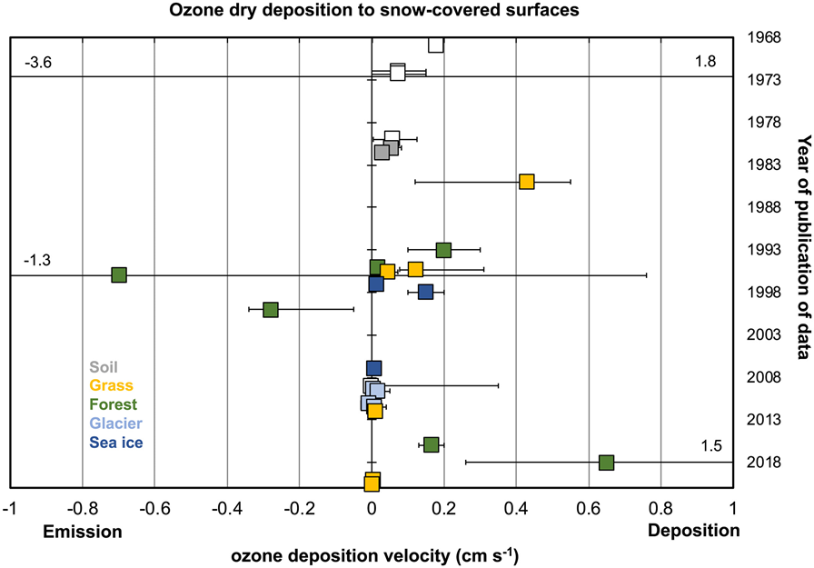
The slowest observed vd are over polar snowpack (both glacial and sea ice), suggesting ozone uptake to snow-covered landscapes is not primarily controlled by snow presence. While ozone destruction by snow grains may be slow, the transport of air through snowpack (a porous medium with high surface area) to the bottom (Helmig, Bocquet, et al., 2007) occurs on timescales of minutes to hours, allowing ozone destruction through reaction with surfaces within or underneath the snowpack. Snow-covered forests exhibit the fastest vd relative to other snow-covered surfaces, followed by snow-covered grassland and soils (Figure 7).
Hypothesized or identified pathways for ozone dry deposition over snow-covered surfaces include reaction with organic or humic trace impurities, black carbon (Albert et al., 2002), and halogens (Peterson & Honrath, 2001). Based on snowpack chemical and transport modeling, reaction with bromine (Thomas et al., 2011) and formic acid in the aqueous phase (Murray et al., 2015) may be ozone deposition pathways for snow on glacial ice. In environments where vegetation protrudes from the snow, ozone uptake by biological materials may be the determining ozone sink.
For seasonally deep snowpack at midlatitudes, snowpack insulates the ground, promoting relatively warm and moist soil conditions that foster soil microbial processes resulting in a steady production and emission of NO. For example, interstitial air is enriched in NO by a factor of up to ~100 compared to the air above the surface at Niwot Ridge (Helmig, Seok, et al., 2009). Snowpack reaction between ozone and NO under low light conditions when NO2 photolysis does not occur may be a primary route for ozone loss in this type of environment. Currently, there are no observations of ozone dry deposition over snow-covered permafrost soils. Such observations may help establish vd over snow-covered soils without the contribution of ozone reaction with NO.
Ozone deposition velocity over snow-covered surfaces also exhibits a diel cycle, with maximum values in the afternoon (Helmig, Cohen, et al., 2009; Neirynck & Verstraeten, 2018). The processes driving the diel cycle are uncertain.
Most models apply a constant resistance for ozone dry deposition to snow regardless of environmental conditions and the substrate underneath the snowpack. As evident from vd variability for snow-covered surfaces (Figure 7), a single resistance does not describe ozone dry deposition over myriad snow-covered environments accurately. A more comprehensive parameterization likely requires accounting for dependencies on snow conditions, chemical snow properties, and substrate underneath snowpack. Variability in observed vd for a given LULC also emphasizes the need for observational constraints.
A range of approaches has been used to study ozone fluxes over snow, including observing ozone decay in chambers filled with snow (Aldaz, 1969; Galbally & Roy, 1980), the flux gradient technique (Bocquet et al., 2011; Colbeck & Harrison, 1985; Helmig, Cohen, et al., 2009; Neirynck & Verstraeten, 2018; Z. Wu et al., 2016), EC (Stocker et al., 1995; Zeller & Hehn, 1996; Zeller & Nikolov, 2000), and near-surface vertical profiles measured with an automated elevator system (Van Dam et al., 2010).
Low snowpack ozone fluxes challenge instrument resolution and thus uncertainty needs to be considered. Snow cover promotes thermal inversions in the surface layer that weaken turbulence and limit the applicability of micrometeorological techniques for flux measurements. Methods for measuring ozone in air withdrawn from snowpack are highly sensitive and promising for constraining the controls on and strength of ozone snowpack sinks (Bocquet et al., 2007; Helmig, Bocquet, et al., 2007; Seok et al., 2015; Van Dam et al., 2015).
Several studies report negative vd over snow-covered surfaces, suggesting emission from the surface (Galbally & Allison, 1972; Zeller & Hehn, 1996; Zeller & Nikolov, 2000). Relatively large negative vd in earlier work has not been reproduced recently (Figure 7), bringing up the question of whether older findings are influenced by earlier experimental approaches with higher uncertainty. We recommend emphasizing newer relative to older measurements due to the improvement of EC instrumentation and refinement of data-analysis protocols.
Recent high-resolution ozone flux measurements show consistently negative (but relatively small) nighttime vd at Summit in Greenland with increasingly negative values toward summer (Helmig, Cohen, et al., 2009). Snowpack is not a location of ozone production: Ozone in snowpack interstitial air is generally depleted compared to above the surface (Albert et al., 2002; Bocquet et al., 2007; Helmig, Bocquet, et al., 2007; Peterson & Honrath, 2001; Seok et al., 2015), and ozone is always destroyed in snow chamber experiments (Aldaz, 1969; Bottenheim et al., 2002). However, ozone production in the poorly mixed layer right above snow may occur following the accumulation of ozone precursor emissions from the snowpack and enhanced irradiance from snow (e.g., Crawford et al., 2001; Cristofanelli et al., 2018; Helmig et al., 2008; Legrand et al., 2009, 2016).
4.6.1 Main Takeaways
- There is strong variability in observed vd over snow-covered surfaces.
- Accurate modeling of ozone dry deposition to snow-covered surfaces requires better understanding of dependencies on underlying substrate, snow conditions, and meteorology.
- We recommend emphasizing relatively newer measurements due to the improvement of EC instrumentation and refinement of data-analysis protocols.
5 Simulating Ozone Dry Deposition in Regional and Global Models
Most ozone dry deposition schemes used in regional and global models employ big-leaf resistance networks (section 3) and rely on lookup tables for component resistances and changes with season and LULC type (e.g., Simpson et al., 2001; Wesely, 1989; L. Zhang et al., 2002). While environmental conditions (e.g., temperature or surface wetness) sometimes modify lookup values, there is rarely mechanistic representation of processes in dry deposition schemes. Incomplete process representation limits the fidelity of these schemes in simulating ozone dry deposition impacts on air pollution, ecosystems, and climate.
Wesely (1989) is the basis of many large-scale models' dry deposition schemes. The Wesely (1989) scheme was designed to represent regional and seasonal average conditions. However, observations from very short time periods at only a few field sites informed Wesely (1989) as well as later schemes (e.g., L. Zhang et al., 2002), calling into question whether climatological vd is represented accurately in these schemes. There is also hardly an emphasis on vd variations on timescales other than seasonal or diel (e.g., daily and interannual) in past scheme development, limiting our understanding of variations in ozone pollution.
Despite the similar structure of commonly used dry deposition schemes, vd varies strongly across models (Bela et al., 2015; Herwehe et al., 2011; Hardacre et al., 2015; Park et al., 2014; Z. Wu et al., 2011). For example, monthly vd varies by ±20% across models in the Task Force on Hemispheric Transport of Air Pollution (HTAP) ensemble (Figure 8). Because most HTAP models identify as employing Wesely (1989), substantial intermodel variation emphasizes the need to critically assess the implementation of a given scheme as well as input uncertainty (e.g., LULC distribution). Strong vd variability across models leads to uncertainty in the tropospheric ozone budget (Wild, 2007) as well as model estimates of ozone pollution (e.g., Hogrefe et al., 2018; Walker, 2014) and plant damage.
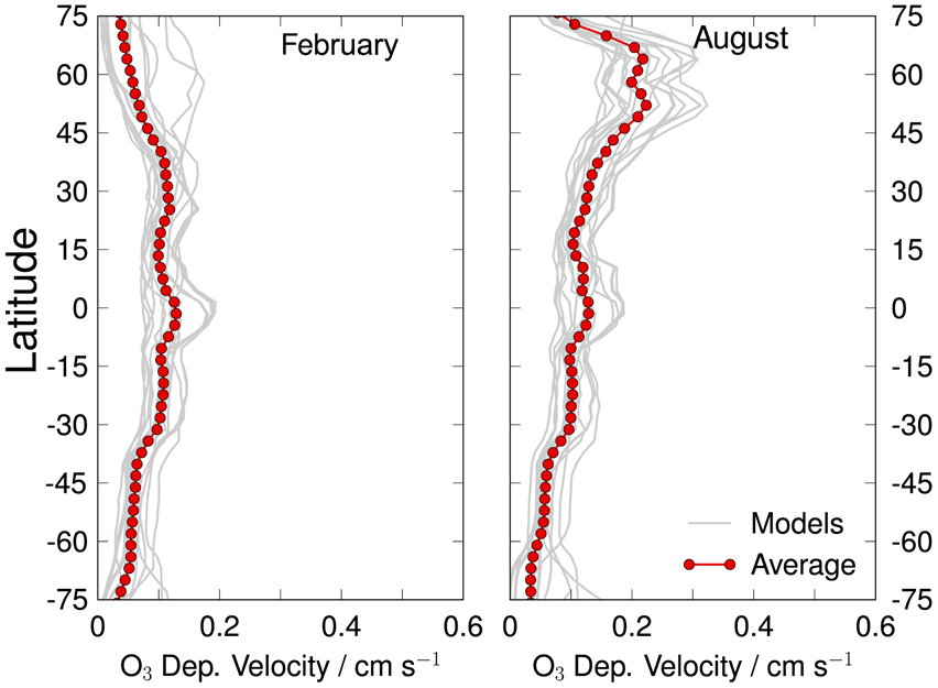
Substantial vd differences also occur among different ozone dry deposition schemes (Schwede et al., 2011; A. Y. H. Wong et al., 2019; Z. Wu et al., 2018). For example, there are twofold to threefold vd differences among five schemes all driven by the same forcing data at Borden Forest in Canada (Figure 9). There are also large differences in summer interannual variability and 30-year trends in vd across four schemes implemented in one global atmospheric chemistry model (A. Y. H. Wong et al., 2019). Studies comparing schemes in depth (Schwede et al., 2011; Z. Wu et al., 2018) illustrate a variety of processes and parameters contributing to intermodel differences.

Improved understanding of parameter and process uncertainty in individual dry deposition schemes (Charusombat et al., 2010; Cooter & Schwede, 2000; Mészáros, Zsély, et al., 2009; Silva & Heald, 2018; Simpson et al., 2003; Tuovinen et al., 2001; Tuzet et al., 2011) is needed and will inform vd differences and similarities across models. We recommend archival of model diagnostics oriented toward processes and LULC types (see Figure 10) in multimodel comparison efforts because such diagnostics allow pinpointing the causes of intermodel similarities and differences.
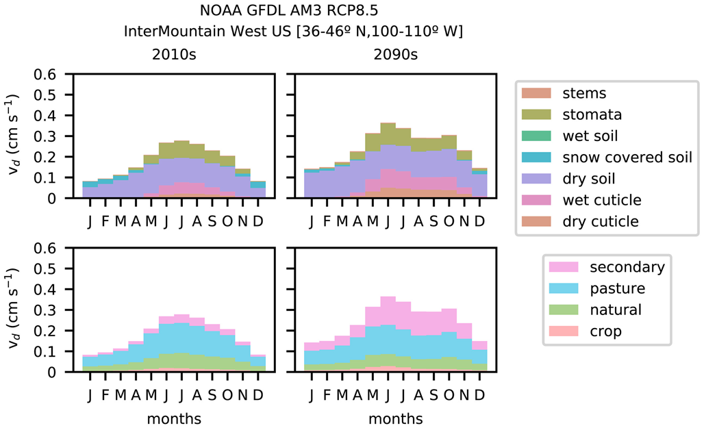
Model ozone dry deposition evaluation typically consists of comparing simulated and observed seasonal vd averages or diel cycles with observations at sites with ozone fluxes (Centoni, 2017; Clifton, 2018; Hardacre et al., 2015; Silva & Heald, 2018; Val Martin et al., 2014; Z. Wu et al., 2018). Some observed climatological features are captured by current schemes. For example, the modified Wesely (1989) scheme in GEOS-Chem captures diel cycles and seasonality at various sites relatively well but does not capture the vd spatial distribution (Silva & Heald, 2018). However, in general, skill varies by model and site, and there is poor understanding of the processes leading to similarities and differences between models and observations (Centoni, 2017; Hardacre et al., 2015; Silva & Heald, 2018; Val Martin et al., 2014; Z. Wu et al., 2011).
Ozone flux data sets used for model evaluation typically span a couple of months at maximum. However, vd varies by a factor of 2 across 11 years of observations at Harvard Forest, which is not captured by the modified Wesely (1989) scheme in GEOS-Chem (Clifton et al., 2017). Strong unreproducible vd interannual variability suggests model evaluation with a single year of observations is inadequate. We recommend emphasizing multiyear averages from long-term ozone flux data sets over short-term data sets for climatological vd evaluation.
Ozone flux data sets are limited to homogeneous terrain (e.g., Wesely & Hicks, 2000), so models are unconstrained for complex terrain. Given that the theories underpinning current parameterizations assume horizontal heterogeneity, models likely perform poorly over complex landscapes.
Future work should evaluate model performance not only in terms of climatological seasonal and diel cycles of vd but also spatiotemporal variability and relationships with meteorological and biophysical parameters. For example, observations suggesting a weak dependence on LAI (Clifton et al., 2017, 2019; Mahrt et al., 1995; Wolfe et al., 2015) may imply the strong LAI sensitivity in many models (Charusombat et al., 2010; Schwede et al., 2011; Silva & Heald, 2018) is exaggerated. However, whether observations generally suggest a weak dependence on vegetation density is unknown; some work suggests a strong dependence (e.g., MacPherson et al., 1995). The most insightful model evaluation relies on process-oriented relationships yet to be identified from a meta-analysis of observations.
Only a few studies probe the roles of deposition processes driving model biases (e.g., Tuovinen et al., 2004; Z. Wu et al., 2018). Most studies largely assume stomatal uptake drives variations in vd. We emphasize the contribution of nonstomatal deposition (Figure 4) should be considered in model evaluation. We recommend developing and archiving model diagnostics oriented toward processes (Figure 10). Isolating simulated vd for a specific LULC type from the grid-box average (Figure 10), which combines multiple LULC types, is also helpful for more direct comparison with observations (e.g., Paulot et al., 2018; Silva & Heald, 2018). For evaluation with such diagnostics to be most instructional, a firm grasp on the relative roles of individual ozone deposition pathways and the mechanisms responsible for differences across LULC types as gleaned from observations is needed.
In general, differences between site and model environmental variables (e.g., meteorology or soil moisture) and observational uncertainty confound model evaluation (Cooter & Schwede, 2000; Schwede et al., 2001; Silva & Heald, 2018; Tuovinen et al., 2001; Z. Wu et al., 2018). To reduce the impact of differences between site and model variables on model evaluation and thus separate input uncertainty from process and parameter uncertainty (e.g., Z. Wu et al., 2018), we recommend driving standalone schemes with observed variables representative of the flux-tower footprint. Given more observational constraints on the processes controlling observed vd, driving models with flux-tower data will allow identification of realistic and robust schemes. Otherwise, as is the case for modeling at regional-to-global scales, agreement with observations may stem from incorrect contributions from the various deposition pathways.
6 Remaining Gaps and Recommendations for Future Work
Ozone dry deposition intersects multiple fields, including atmospheric chemistry, plant physiology/ecology, and boundary-layer meteorology, all with distinct research questions on the subject (e.g., Hosker & Lindberg, 1982). While ecologists aim to quantify stomatal ozone uptake and understand the ensuing damage to plants, atmospheric chemists aim to quantify ozone deposition velocity over different surfaces and understand the impact of ozone dry deposition on tropospheric chemistry and composition. Identifying current measurement techniques, modeling, and available data as well as assessing and advancing knowledge on ozone dry deposition requires bridging across distinct research communities.
Current understanding of ozone dry deposition is largely based on only a few ozone flux data sets, many of which only span short time intervals. It is generally uncertain which aspects of observed ozone dry deposition are specific to a given site versus represent the broader region or LULC type or are climatological versus episodic. Our top recommendation is establishing key field sites with long-term ozone EC fluxes. The highest priority complementary measurements depend on the specific question ranked as most important (Table 4). If robust evaluation of variability across sites is a desired outcome of future field studies, then a coordinated approach across sites is needed to ensure consistency across measurements.
| What is the contribution of stomatal uptake to ozone dry deposition?* | Water vapor flux, carbon dioxide flux, friction velocity | Other independent tracers of stomatal conductance (e.g., carbonyl sulfide flux) and canopy skin temperature |
| What is the contribution of leaf cuticular uptake to ozone dry deposition? | Humidity, leaf/canopy wetness, leaf area index, dew point temperature, precipitation, same as * to obtain residual ecosystem-scale nonstomatal conductance | Chamber fluxes for ozone around branches including tracers of stomatal conductance to isolate cuticular uptake and composition of cuticles |
| What is the contribution of soil uptake to ozone dry deposition? | Soil moisture and temperature, same as * to obtain residual ecosystem-scale nonstomatal conductance | Lower canopy ozone fluxes, fluxes of NO, NO2, and highly reactive BVOC emission from soil, chambers measuring ozone uptake by soil, and soil properties (e.g., organic content, clay content, porosity, and hydraulic conductivity) |
| What is the contribution of chemistry in the canopy air space to ozone dry deposition? | NO and NO2 fluxes, highly reactive BVOC fluxes, same as * to obtain residual ecosystem-scale nonstomatal conductance | Fluxes of oxidation products |
| How do snow-covered surfaces influence ozone dry deposition? | Horizontal and vertical extent of snow cover, snow age | Snow impurities and NO content of snowpack |
We also recommend that older data sets be revisited in order to build on the deeper mechanistic understanding revealed by our synthesis here. Our efforts to document ozone flux records since 1985 identifies over 100 sites with measurements. A central archive of ozone fluxes along with complementary data would facilitate broad synthetic meta-analyses and hasten progress toward robust scientific advances. Quantifying uncertainty in data, particularly with respect to random and systematic errors associated with measurement technique, is essential when synthesizing information across data sets. We suggest holistic examinations of older data sets will lead to new knowledge of the processes and conditions driving ozone dry deposition on different temporal and spatial scales.
Because there are only a handful of sites with long-term ozone flux records and many no longer measure ozone fluxes, we emphasize that continued support of current and past sites and establishment of new long-term sites are fundamental to advance knowledge. Because ozone dry deposition is closely related to carbon and water exchange and associated conditions (e.g., ambient humidity and soil organic content), science will progress most rapidly when ozone fluxes are added to sites already well characterized in terms of carbon and water cycling and boundary-layer meteorology.
For both future short-term campaigns and long-term monitoring, we recommend measuring ozone flux through ozone EC. That the fast ozone analyzers required for ozone EC either require frequent maintenance or are expensive and require toxic or flammable compressed gases is a potential roadblock. We emphasize the importance of developing new analytical methods for fast ozone measurement. An effort to coordinate across research groups measuring ozone fluxes is sorely needed and should promote best practices learned from the carbon dioxide flux community in calculating fluxes, filtering data sets, and sharing data. Such an effort should also include validation and intercomparison of different fast ozone analyzers.
While our review offers an unprecedented synthesis of process-based knowledge of ozone deposition pathways, the relative importance of individual depositional pathways remains uncertain. In particular, we emphasize large uncertainty in the partitioning of ozone dry deposition occurring through pathways other than through plant stomata. Our synthesis of observationally based estimates of the stomatal fraction of ozone dry deposition across peer-reviewed literature shows on average the stomatal fraction over physiologically active vegetation is 45%, underscoring the importance of nonstomatal deposition.
Process-oriented investigation of spatiotemporal variations and trends in ozone fluxes is necessary to quantify the relative importance of various deposition pathways and will inform the degree of complexity needed to model deposition of ozone at large scales. If coordinated with short-term field intensives, laboratory studies, and mechanistic modeling, measurements from a few long-term sites as described in Table 4 would bridge the molecular to ecosystem scales needed to establish the relative importance of various deposition pathways and the extent to which they vary in space and time.
Advancing understanding of dry deposition of ozone is also relevant for dry deposition of other reactive trace gases that alter atmospheric chemistry, climate, and ecosystems because similar physical and chemical processes govern their uptake. Process knowledge of dry deposition for ozone can be translated to any trace gas that reacts with surfaces (e.g., nitrogen dioxide or oxygenated volatile organic compounds). Additionally, models frequently parameterize dry deposition of other reactive trace gases by using ozone and sulfur dioxide as end members. Specifically, a gas's oxidizing ability is scaled to ozone dry deposition, while a gas's solubility is scaled to sulfur dioxide dry deposition given ozone is an oxidant but insoluble and sulfur dioxide is not an oxidant but soluble. Building on the mechanistic framework for ozone dry deposition outlined in this review should inform the strengths and limitations of such a parameterization.
The optimal parameterization for ozone dry deposition remains elusive, but the process understanding synthesized in this review lays the groundwork for one. Representation of most deposition processes in current models should be regarded as insufficient. While current parameterizations capture some of the main observed features of ozone dry deposition, the underlying brazen empiricism of these schemes hinders a full mechanistic understanding of the influence of ozone dry deposition on air pollution, ecosystems, and climate.
Acknowledgments
This material is based upon work supported by the National Center for Atmospheric Research, which is a major facility sponsored by the National Science Foundation under Cooperative Agreement 1852977. O. E. C. also acknowledges support from an NSF Graduate Research Fellowship (DGE 16-44869). A. M. F. acknowledges funding from NOAA's Climate Program Office's Atmospheric Chemistry, Carbon Cycle, and Climate program Grant NA14OAR4310133. O. E. C. acknowledges conversations with participants from a workshop on ozone dry deposition at Lamont-Doherty Earth Observatory in October 2017. The full list of participants in this workshop is given in Appendix C. The workshop was supported by the Lamont Climate Center, NASA, and NOAA. O. E. C. is also grateful for conversations with Róisín Commane, Adriana Bailey, and Andrew Weinheimer and thanks Don Lenschow, Jonathan Pleim, and Robert Pinder for comments on the manuscript. Disclaimer: The views expressed in this article are those of the authors and do not necessarily represent the views or policies of the U.S. Environmental Protection Agency. Data sets generated for Figures 2, 3, 4, 7, and 10 are available online (https://doi.org/10.5065/w2zc-bt87). Other figures containing scientific data are reprinted from the peer-reviewed literature: S. Sun, Morvakev, Trebs, et al. (2016) for Figure 6, Hardacre et al. (2015) for Figure 8, and Z. Wu et al. (2018) for Figure 9. O. E. C. thanks three anonymous reviewers for their constructive comments on this manuscript.
Appendix A: Ecosystem-Scale Ozone Flux Data Sets
Appendix A contains the table of ecosystem-scale ozone flux data sets from 1985 onward.
| Alice Holt | England | 51.17°N | 0.87°W | July–August 2005 | EC | Oak forest | |
| Amazon Tall Tower Observatory | Brazil | 2.1459°S | 59.00°W | December 2015 and March 2016 to present | EC | Tropical forest | |
| Auchencorth Moss | Scotland | 55°47′30″N | 3°14′20″W | 1995–1998 | Gradient | Moorland | Fowler et al. (2001) and Tuovinen et al. (2004) |
| Beaufort | Southeast United States | 34.88°N | 76.62°W | 10 June to 1 August 1993 | EC | Crop | Finkelstein et al. (2000) and Meyers et al. (1998) |
| Beijing | China | 39.98°N | 116.39°E | August–November 2016 and May–June 2017 | EC | Urban | |
| Bergamo | Italy | 45°36′51″N | 9°40′22″E | May–June 2001 | EC | Wheat field | Gerosa et al. (2003) |
| Bily Kriz | Czech Republic | 49°33′N | 18°32′E | July–August 2008 and 2012–2017 (gradient), summer 2017 (EC) | EC and gradient | Norway spruce forest, established in 1981 by planting 4-year-old seedlings in rows | Juráň et al. (2019) and Zapletal et al. (2011) |
| Blodgett Forest | California | 38.9°N | 120.63°W | June–September 1997, May–November 1998, June 1999 to June 2000, and January 2001 to December 2006 | EC | Ponderosa pine plantation | Bauer et al. (2000), Fares, McKay, et al. (2010), Goldstein (2003), Goldstein et al. (2004), Kurpius et al. (2002), Kurpius and Goldstein (2003), and Wolfe et al. (2011) |
| Bondville | Midwest United States | 40.05°N | 88.37°W | 18 August to 1 October 1994 | EC | Corn | Finkelstein et al. (2000), Finkelstein (2001), Meyers et al., (1998), Y. Wu, et al. (2003), and L. Zhang, et al. (2002) |
| Bosco Fontana | Italy | 45°12′02″N | 10°44′44″E | 12 June to 11 July 2012 | EC | Mixed oak-hornbeam forest | Finco et al. (2018) |
| Braunschweig | Germany | 53°18′N | 10°26′E | 20 May to 15 June 2000 | EC | Intensively managed grassland | Bassin et al. (2004) and Mészáros, Horváth, et al. (2009) |
| Bruneck | Italy | 46°49′N | 11°55′E | December 1999 | EC | Snow-covered mountain valley | Cieslik (2009) |
| Bugacpuszta | Hungary | 46.69°N | 19.60°E | August 2012 to January 2014 | EC | Seminatural semiarid sandy grassland | Horváth et al. (2017) |
| Bukit Atur | Malaysia | 4°58′49.10″N | 117°51′19.12″E | 7 April to 24 July 2008 | EC and gradient | Tropical forest | Fowler et al. (2011) |
| Burriana | Spain | 39°55′N | 0°03′W or 0.04′W | 16–29 July 1995, 28 April to 3 May 1996, and 2–16 June 1997 | EC | Orange grove | Cieslik (2004) |
| Cala Violina | Italy | 42°55′N | 10°30′E | June–December 2005 and July–September 2006 | EC | Mixed oak forest in complex terrain | Cieslik (2009) and Gerosa et al. (2007) |
| Camp Borden | Canada | 44°19′N | 79°56′W | July–August 1988 (EC), March–April 1990 (EC), and May 2008 to April 2013 (gradient) | EC and gradient | Temperate mixed forest | Fuentes et al. (1992), Padro (1993, 1994), Padro et al. (1991), and Z. Wu et al. (2016, 2018) |
| Castelporziano | Italy | 41.42°N | 12.21°E | June 1993 and May 1994 | EC | Mediterranean pseudo steppe | Cieslik (2004) and Cieslik and Labatut (1997) |
| Castelporziano | Italy | 41.42°N | 12.21°E | August–September 2003, June–November 2004, June–October 2003, and 2011–2015 | EC | Holm oak forest | Gerosa et al. (2005, 2007), Gerosa, Finco, Mereu, Marzuoli, et al. (2009), Fares et al. (2013, 2014), Hoshika et al. (2017), Rydsaa et al. (2016), Savi and Fares (2014), and Vitale et al. (2005) |
| Castile and Leon | Spain | 42°1′N | 4°32′W | 5, 6, and 8 May 1994 and 6 days in July 1995 | Gradient | Semiarid steppe on a plateau covered in barley | De Miguel and Bilbao (1999) and Sánchez et al. (1997) |
| Central Plains Experimental Range | Western United States | 40°28′23″N | 104°45′15″W | 5 March to 2 August 1988, 24 January to 21 February 1989, and 7 June to 10 July 1989 | EC | Bare patches of soil and dead or senescent vegetation or snow | Massman (1993) and Stocker et al. (1993, 1995) |
| Chinese Research Academy of Environmental Sciences | Beijing | September and November 2000, 10 days each | Gradient | Grassland | Sorimachi et al. (2003) | ||
| CODE cotton | California | 36°48′50″N | 120°40′38″W | 8 July to 6 August 1991 | EC | Cotton | Grantz et al. (1997), Massman et al. (1994), Padro et al. (1994), and Padro (1996) |
| CODE grassland | California | 37°02′N | 119°48′30″W | 30 days during summer 1991 | EC | Grassland | Massman et al. (1994), Padro, Massman, Shaw, et al. (1994), and Padro (1996) |
| CODE vineyard | California | 36°51′36″N | 120°6′7″W | 11 July to 1 August 1991 and 8 July to 6 August 1991 | EC | Grape | Grantz et al. (1995), Massman et al. (1994), Padro, Massman, Den Hartog, et al. (1994), and Padro (1996) |
| Colt Park | England | 54.19°N | 2.34°W | August to October 2005 | EC | Seminatural grassland | |
| Comun Nuovo | Italy | 45°37′N | 9°40′E | May–June 2001, July–September 2001, and May–June 2002 | EC | Wheat, soybean, or barley | Bassin et al. (2004), Cieslik (2009), Gerosa et al. (2003), Tuovinen et al. (2004), and Rydsaa et al. (2016) |
| Cuatro Vientos | Spain | 40°40′N | 3°56′W | 2–13 May 1997 | EC | Low vegetation | Cieslik (2004) |
| Dakhla Oasis | Egypt | 23 March to 9 April 1993 | EC | Saharan desert | Güsten et al. (1996) | ||
| Diepoholz | Germany | 52°39′8″N | 8°39′12″E | 30 June to 4 August 2014 | EC | Peatland | El-Madany et al. (2017) |
| Duke Forest | Southeast United States | Spring 2017 to 2019 | EC | Bottomland mixed hardwood forest along urban to rural gradient | |||
| Duke Forest Blackwood Division | Southeast United States | 35.97°N | 79.13°W | 15 April to 15 May 1996 | EC | Loblolly pine plantation | Finkelstein et al. (2000) and Meyers et al. (1998) |
| Easter Bush | Scotland | August 2007 | EC | Grasslands with predominately perennial rye-grass with grazing in adjacent fields | Muller et al. (2009, 2010) | ||
| Flanders | Belgium | 51°18′N | 4°31′E | 2000–2015 | Gradient | Mixed forest in a suburban area | Neirynck et al. (2012) and Neirynck and Verstraeten (2018) |
| Gilchriston Farm | Scotland | 55.9°N | 2.8°W | 1 month in summer 2006 | EC | Potato canopy | Coyle et al. (2009) |
| GLEES Brooklyn Lake | Western United States | 41°22′N | 106°14.5′W | 14–27 April, 6–19 May, June, and 2–9 July 1992, 15–26 January 1993, and 30 July to 8 August 1996 | EC | Subalpine coniferous forest | Zeller (2000), Zeller and Hehn (1995, 1996), and Zeller and Nikolov (2000) |
| GLEES Brooklyn Lake | Western United States | 41°22′N | 106°14.5′W | 24 April to 3 May 1994, and 7–21 June and 2–10 August 1994 | EC | Open meadow | Zeller and Hehn (1995) |
| Grignon | France | 48.84°N | 1.95°E | 19 June to 7 October 2002, 26 July to 1 October 2002, 2004–2009, and 7 August 2012 to 13 March 2013 | EC | Crop (sometimes bare soil, maize, and winter wheat) | Lamaud et al. (2009), Loubet et al. (2013), Stella, Loubet, et al. (2011), Stella, Personne, et al. (2011), Stella et al. (2012, 2013, 2019), Tuzet et al. (2011), and Vuolo et al. (2017) |
| Halvergate Trace Gas Exchange Experiment | England | 15 September 1989 | Gradient | Drained marshland pasture | Hargreaves et al. (1992) and Kramm et al. (1991) | ||
| Hartheim | Germany | 47°56′N | 7°37′E | 17–20 May 1992 | Gradient | Scots pine plantation | Joss and Graber (1996) |
| Harvard Forest | Northeast United States | 42.53°N | 72.18°W | 1990–2000 | EC and gradient | Temperate deciduous forest | Clifton et al. (2017, 2019), Munger et al. (1996), and Z. Y. Wu et al. (2015) |
| Hesse | France | 48°0′27″N | 7°03′52″E | September 2010 to March 2011 | EC | European beech | Le Morvan-Quéméner et al. (2018) |
| Hohenpeissenberg | Germany | 47°48′N | 11°02′E | 29 August to 20 September 2005 | EC | Meadow and pre-alpine landscape | Stella et al. (2013) |
| Horsepool | Western United States | 25 January to 2 April 2013 | EC | Dry, sandy soil and low-lying sage brush | |||
| Hortobágy | Hungary | 19–30 June 1993, 5 May to 21 June 1994, and 13–30 September 1994 | Gradient | Grassland | Horváth et al. (1997) | ||
| Hurdal | Norway | 1 July 2000 to 31 March 2003 | Gradient | Norway spruce forest | Hole et al. (2004) | ||
| Hyytiälä | Finland | 61.85°N | 24.28°E | 2001–2013 | EC | Coniferous forest | Altimir et al. (2006), Launiainen et al. (2013), Rannik et al. (2009, 2012), and P. T. Zhou et al. (2017) |
| Ispra forest | Italy | 45.8126°N | 8.6336°E | 2013–2015 | EC | Deciduous forest | |
| Ispra grassland | Italy | 44°48′N | 8°38′E | September 1997 | EC | Grassland | Cieslik (2009) |
| Kaamanen | Finland | 69°08′N | 27°17′E | September 1995 | EC | Open fark fen (ridges and open water pools) | Tuovinen et al. (1998, 2004) |
| Kane Experimental Forest | Northeast United States | 41.60°N | 78.77°W | 29 April to 23 October 1997 | EC | Deciduous forest | Finkelstein et al. (2000), Finkelstein (2001), Meyers et al. (1998), L. Zhang et al. (2001, 2002) |
| Keenly Fell | England | 54°53′49.0″N | 2°19′26.6″W | June 2007 to December 2011 | EC | Seminatural grassland | |
| Klippeneck | Germany | 48°10′N | 8°45′E | 10–22 September 1992 | Grassland | Cieslik (2004) | |
| Konza Praire Research Natural Area | Central United States | 26 May to 6 June 1987, 25 June to 11 July, 6–21 August 1987, and 5–16 October 1987 | EC | Predominately big bluestem grass; recent fire | Gao et al. (1992) | ||
| Kranzberger Forst | Germany | 48°25′N | 11°39′E | 2–29 July 2007 | EC | Mixed forest | Nunn et al. (2010) |
| La Barben | France | 43°35′N | 5°15′E | 29 June to 13 July 2001 | EC | Mediterranean shrubland, mostly Quercus coccifera | Michou et al. (2005) |
| La Cape Sud | France | 44°24′N | 0°38′W | 26 July 2007 to 4 March 2008 | EC | Crop | Stella, Personne, et al. (2011) and Stella et al. (2019) |
| La Crau | France | 43°34′N | 4°49′E | 20 April to 31 May 2001 | EC | Semiarid part of the La Crau plain and totally flat, uniform, almost bare soil with mainly pebbles | Michou et al. (2005) and Stella et al. (2019) |
| Lake Kinisheo | Canada | Late June to July 1990 | Lichen bogs and small conifer shrubs | Fuentes et al. (1994) | |||
| Lake Kuivajärvi | Finland | 61°50′N | 24°17′E | August to September 2012 | EC | Boreal lake | Fung (2018) |
| Lamasquére | France | 43°49′N | 1°23′W | 2008–2010 | EC | Crop | Stella, Personne, et al. (2011) and Stella et al. (2019) |
| Le Bray | France | 44°34′33.24″N | 0°46′33.72″W | May to August 2007 and May to August 2008 | EC | Stand of maritime pines planted in 1970 | Le Morvan-Quéméner et al. (2018) |
| Le Dézert | France | 44°05′N | 0°43′W | 16–18 April 1997 | EC | Coniferous forest | Cieslik (2004) |
| Les Landes | France | 44°12′N | 0°42′W | June 1994, 21 June to 3 July 1997, 21–24 February 1997, June 1996, and October 1996 | EC and gradient | Mixed forest | Lamaud et al. (2002) and Sánchez et al. (1997) |
| Lincove | California | 36.36°N | 119.09°W | October 2009 to November 2010 | EC | Orange orchard | Fares et al. (2012) |
| Lochristi | Belgium | 51°06′44″N | 3°51′02″E | 2010–2016 | EC | Short-rotation coppice poplar plantation | Zenone et al. (2016) and Zona et al. (2014) |
| London | England | 51.52°N | 0.14°W | October 2011 to August 2013 | EC | Urban | |
| Lusignan | France | 46°24′N | 0°07′E | 17 March to 5 May 2011 | EC | Crop | Stella et al. (2019) |
| Lusignan | France | 46°26′08″N | 0°07′25″E | August to September 2010 | EC | Meadow | Le Morvan-Quéméner et al. (2018) |
| Manaus | Brazil | 3°S | 60°W | At most a couple of days in July–August 1985 | Gradient | Tropical forest | Kirchhoff et al. (1988) |
| Mea Moh | Thailand | 18.28°N | 99.72°E | January–April 2002 and January–August 2004 | Gradient | Teak forest | Matsuda et al. (2005, 2006) |
| Mekrijärvi | Finland | 62°52′N | 30°55′E | July 1995 | EC | Low Scots pine forest on border of southern and middle boreal zones | Tuovinen et al. (2001, 2004) |
| Meyrargues | France | 43°39′N | 5°32′E | 12–28 June 2001 | EC | Maize | Michou et al. (2005) |
| Monmeyan | France | 43°39′N | 6°05′E | 10–26 June 2001 | EC | Mediterranean forest (95% Quercus Pubescens) | Michou et al. (2005) |
| Nashville/Keysburg | Southeast United States | 36.65°N | 87.03°W | 22 June to 11 October 1995 | EC | Soybean | Finkelstein et al. (2000), Finkelstein (2001), Meyers et al. (1998), Pleim et al. (2001), Y. Wu et al. (2003), and L. Zhang et al. (2002) |
| Neustift | Austria | 47°07′N | 11°19′E | 11 July to 20 October 2008 | EC and gradient | Temperate mountain meadow | Wohlfahrt, Hörtnagl, et al. (2009) |
| Niwot Ridge | Western United States | 40.03°N | 105.55°W | 6 June to 31 August 2002, 1 April to 19 November 2003, 21 May to 30 June 2004, and 20 May to 31 August 2005 | EC | Coniferous subalpine forest | Turnipseed et al. (2009) |
| Norwood Park | England | 25–28 July 1994 | EC | Fruit orchard | Walton, Gallagher, Choularton, et al. (1997) and Walton et al. (1997) | ||
| Nyírjes | Hungary | 5–30 September 1991, 20 March to 16 April 1992, 28 January to 17 February 1993, 8 July to 29 August 1993, and 15 July to 6 August 1994 | Gradient | Norway spruce forest | Horváth et al. (1997) | ||
| Oshiba Highland | Japan | 32°52′N | 137°58′E | April–September 2001 | Gradient | Red pine forest | S. Zhang et al. (2005) |
| Palatinate | Germany | 49.16°N | 8.28°E | April–September 1992 | EC | Barley or flat harvested field | Güsten et al. (1997) |
| Petsikko | Finland | 69°52′N | 27°14′E | Beginning of June to August 18 1996 | EC | Subarctic mountain birch | Tuovinen et al. (2001) |
| Plymouth | Southeast United States | 35.70°N | 76.80°W | 15 July to 15 August 1996 | EC | Soybean | Finkelstein et al. (2000), Meyers et al. (1998), and Y. Wu et al. (2003) |
| Polder Piloto de Sarazola | Portugal | 40°42′N | 8°37′W | November 1994 to October 1995 | Gradient | Meadow | Pio and Feliciano (1996), Pio et al. (2000), and Tuovinen et al. (2004) |
| Ramat Hanadiv Nature Park | Israel | 32°33′19.87″N | 34°56′50.23″E | 31 July to 30 September 2015, 1 February to 31 March 2016, 1 June to 7 July 2016, 2 August to 17 September 2016, 5 January to 22 May 2017, and 12 June to 2 July 2017 | EC | Shrub 3.6 km away from eastern Mediterranean seashore | Q. Li, Gabay, et al. (2018) |
| Reserve Adolfo Ducke | Amazonia | 2°57′S | 59°57′W | 22 April to 8 May 1987 | EC | Tropical forest | Fan et al. (1990) |
| Rhine Valley | Germany | September 1992 | Gradient | Short sparse wheat | Horváth et al. (1998) | ||
| Rhineland-Palatinate | Germany | 49.9685°N | 8.1481°E | July–October 2011 | EC | Natural nutrient-poor steppe-like grassland and occasionally subject to management in past | Ermel et al. (2013) and Plake, Stella, et al. (2015) |
| Rivox | Scotland | 55°19′57″N | 3°31′43″W | May 1992 | EC | Sitka spruce plantation | Coe et al. (1995) |
| Rondonia | Amazonia | 10°04′55″S | 61°55′48″W | 4–22 May 1999 and 21 September to 20 October 1999 | EC | Wet and dry season, la Niña year | Rummel et al. (2007) |
| Rondonia | Amazonia | 10°45′44″S | 62°21′27″W | 30 April to 17 May 1999 and 24 September to 27 October 1999 | EC | Pasture and transition seasons “wet-dry” and “dry-wet,” la Niña year | Kirkman et al. (2002) and Rummel et al. (2007) |
| S. Pietro Capofiume | Italy | 44°39′N | 11°37′E | 2–11 June 1993 | EC | Beet | Cavicchioli et al. (1997) and Cieslik (2004, 2009) |
| Sabah | Malaysia | 5°14′58.69″N | 118°27′15.76″E | 4–11 June 2008 | EC | Crop | Fowler et al. (2011) |
| San Rossore | Italy | 43°43′55″N | 10°17′27″E | 20 January to 10 February 2013, 22 April to 12 May 2013, 8–27 July 2013, and 9–29 September 2013 | EC | Coniferous forest (Pinus pinea) | Hoshika et al. (2017) |
| Sand Flats State Forest | Northeast United States | 43.57°N | 75.24°W | 12 May to 20 October 1998 | EC | Mixed forest | Finkelstein et al. (2000), Finkelstein (2001), Meyers et al. (1998), and L. Zhang et al. (2002, 2001) |
| Sand Mountain | Southeast United States | 34.29°N | 85.97°W | 15 April to 13 June 1995 | EC | Grassland | Finkelstein et al. (2000), Finkelstein (2001), Meyers et al. (1998), Y. Wu et al. (2003), and L. Zhang et al. (2002) |
| Schachtenau | Germany | June to September 1987 and 18–28 September 1989 | EC | Coniferous forest | Enders (1992) and Enders et al. (1992) | ||
| Schefferville | Canada | 54°50′N | 66°40′W | July to August 1990 | EC | Spruce woodland | Munger et al. (1996) |
| Scherzheim | Germany | 11–22 September 1992 | EC | Harvested and harrowed wheat field with regrown wheat | Pilegaard et al. (1998) | ||
| Sinderhoeve | Netherlands | 51.58°N | 5.42°E | 30 June 1988, 6, 19, 25, and 28 July 1988, 12 and 28 August 1988, 12 and 22 September 1988, and 4 October 1988 | EC | Maize | Van Pul and Jacobs (1994) |
| Speulderbos | Netherlands | 9 months in 1993 | EC | Douglas fir plantation | Dorsey et al. (2004) and Duyzer et al. (1995) | ||
| Summit | Greenland | 72.34°N | 38.29°W | 19–30 July 2003, 22 March to 14 August 2004, and 17 March to 28 April 2005 | Gradient | Polar snowpack on glacial ice | Helmig, Bocquet, et al. (2007) and Helmig, Cohen, et al. (2009) |
| Toolik Lake | Alaska | 68.6°N | 149.6°N | May–August 2011 | EC | Tundra | Van Dam et al. (2016) |
| Turro | Italy | 44°59′N | 9°42′E | March–April 2014 | EC | Crop | Stella et al. (2019) |
| Ulborg | Denmark | 56°17′N | 8°25′E | 7 days in April 1995, 10 days in June 1994, 7 days in August 1997, 5 days in September 1995, and May–June 1995, 2003 (EC) and 1994–2000 (gradient) | EC and gradient | Mixed forest (mostly Norway spruce) | Mikkelsen et al. (2000, 2004), Pilegaard et al. (1995), Ro-Poulsen et al. (1998), and Tuovinen et al. (2004) |
| UMBS Prophet | Midwest United States | 45.5°N | 84.7°W | 27 June to 28 September 2002, 7 August to 15 October 2003, 15 June to 15 September 2004, and 15 June to 3 September 2005 | EC | Mixed forest (bigtooth aspen, white pine, red oak, red maple, and paper birch) | Hogg et al. (2007) and Hogg (2007) |
| Viols-en-Laval | France | 43°41′N | 3°47′E | 16–24 July 1998 | EC | Mediterranean shrub | Cieslik (2004) |
| Virginia Forest Research Facility | Southeast United States | 37.92°N | 78.27°W | July 2019 to present | EC | Mixed forest | |
| Voghera | Italy | 45°01′N | 9°00′E | May–July 2003 | EC | Onion | Cieslik (2009) and Gerosa et al. (2007) |
| Yucheng Comprehensive Experimental Station of the Chinese Academy of Sciences | China | 36°50′N | 116°34′E | 9 August to 28 September 2011 and 2 March to 6 June 2012 | EC | Corn and wheat | Zhu et al. (2014) and Zhu (2019) |
| Yukon Delta National Wildlfie Refuge | Alaska | 61°05.41′N | 162°00.92′W | 14 July to 12 August 1988 | EC | Tundra | Jacob et al. (1992) |
| Zegveld | Netherlands | 6 September 1994 | Gradient | Dutch pasture | Galmarini et al. (1997) |
Appendix B: Mechanistic Modeling
1 Mechanistic Modeling of Ozone Dry Deposition to Leaf Cuticles
Here we derive and review the Potier et al. (2015) physically based model for ozone dry deposition to wet leaves. We begin with the steady-state diffusion/reaction equation for aqueous ozone (O3,aq) (mol m−3):
This rcut,wet expression is the same as Potier et al. (2015) equation (A5) except for our using the dimensionless form of Henry's law constant.
B.2. Mechanistic Modeling of Ozone Dry Deposition to Soil
However, soils vary vertically in terms of η, τ, θ, and temperature (Tsoil), which may influence variables such as
.
The next steps are to construct
and
. We parameterize
as
where
(ppmv s−1) is the rate coefficient for ozone chemical destruction in soil pore spaces by some gas species Xsoil.